Quantcast
Channel: elasticsearch – Neo4j Graph Database Platform
Viewing all 32 articles
Browse latest View live

The Future of Recommendation Engines: Graph-Aided Search

$
0
0
Learn How the Future of Real-Time Recommendation Engines Merges with Graph-Aided Search
Learn How the Future of Real-Time Recommendation Engines Merges with Graph-Aided SearchEditor’s Note: GraphAware is a Silver sponsor of GraphConnect San Francisco. Register for GraphConnect to meet Michal and other sponsors in person.

For the last couple of years, Neo4j has been increasingly popular as the technology of choice for people building real-time recommendation engines.

Having been at the forefront of the graph movement through client engagements and open source software development, we have identified the next step in the natural evolution of graph-based recommendation engines. We call it Graph-Aided Search.

Recommendation Engines Everywhere


At first glance, it may seem that graph databases are only good for social networks, but it has been proven over and over again that the variety of domains and industries that need a graph database to store, analyse and query connected data could not be any wider.

Similarly, recommendation engines go far beyond retail – the most obvious industry. We’ve seen real-time recommendations with Neo4j applied to finding:

    • Matches on dating sites (Dating, Social)
    • People one may know in professional networks (Social)
    • Ideal candidates for clinical trials (Pharma)
    • Fraudsters (Banking, Insurance, Retail)
    • Criminals (Law Enforcement)
    • Events of interest (Event Planning)
    • And many more

Real-Time Recommendations


The reasons for wanting to implement a system that serves recommendations in real-time and for choosing a native graph database to do that have been well understood and written about.

Once the technology choice has been made, there are three main challenges to building such a recommendation engine. The first one is to discover the items to recommend. The second is to choose the most relevant ones to present to the user. Finally, the third challenge is to find relevant recommendations as quickly as possible.

Typically, the input to the recommendation engine is an object (e.g., a user) for which we would like to determine the recommendations. Such an object is represented in the graph as a node, so the whole process is effectively a traversal through the network, finding paths from the input node to other nodes, some of which will be deemed as the most relevant ones and served as recommendations.

Last year, GraphAware built an open source recommendation engine skeleton that runs as a Neo4j extension and provides a foundation to address the three challenges outlined above.

It does so by allowing developers to plug in their (path-finding) business logic into a best-practice architecture, resulting in a fast, flexible, yet simple and maintainable piece of software. The architecture imposes the separation of concerns between the plug-in components that:

    • Discover all possible recommendations
    • Apply a score to the identified recommendations
    • Filter out irrelevant or blacklisted recommendations
    • Optionally record why and how fast the recommendations were served
The skeleton is responsible for sorting by relevance, performance optimisations, thread-safety and other “frameworky” features.

Since its first release, the GraphAware Recommendation Engine has been used by teams all around the world to build production-ready recommendation functionality into their applications.

Search Engines


The vast majority of websites and other systems today provide some sort of search capability, allowing users to find what they are looking for very quickly. Lucene-based search engines, such as Elasticsearch and Apache Solr are the leading technologies in this space.

Like recommendation engines, search engines also serve results in real-time, sorted by decreasing relevance. However, the input to these systems is typically a string of characters and the results are matching documents (items).

Without adding extra complexity, the user performing the search is not taken into account. Hence, two users searching for the same thing will get the same results.

Graph-Aided Search


For the same reasons people are interested in personalising recommendations, they also want to personalise search results.

To see an example of such personalisation in practice, just head to LinkedIn and type the first name of one of your connections into the search box. Your connections will appear on top of the results. Not because they are the most important person with that first name on LinkedIn, but because they are most likely the person you are looking for.

One can treat such functionality as a recommendation engine with all candidate recommendations provided by an external system (search engine in this case), as opposed to discovered by the recommendation engine itself.

Applying the “right tool for the job” philosophy, we can use the search (S) and recommendation (R) engines together to achieve what we call Graph-Aided Search:

    • Discover all matching recommendations (S)
    • Apply a score to the recommendations based on textual match (S)
    • Apply a score to the recommendations based on the user’s graph (R)
    • Filter out irrelevant or blacklisted recommendations (R)
This way, the power of both systems can be used to build personalised search functionality.

Learn More at GraphConnect


At GraphAware, we are currently finalising the development of enterprise-ready extensions to Neo4j and Elasticsearch for bi-directional integration of the two systems, so that they can be easily combined to provide Graph-Aided Search.

We will launch and open source both extensions at this year’s GraphConnect San Francisco.

If you are interested in real-time recommendations, personalising search results or integrating Neo4j with a search engine such as Elasticsearch, come see my presentation at GraphConnect, starting at 2:20 p.m.


Register to hear Michal Bachman’s presentation on real-time recommendation engines and the future of search – along with many other industry-leading presentations – at GraphConnect San Francisco on October 21st.


GraphGrid Interview: Neo4j for Your Modern Graph Data Architecture

$
0
0
Read This Interview with the Co-Creators of GraphGrid about Neo4j for Your Graph Data Architecture
Read This Interview with the Co-Creators of GraphGrid about Neo4j for Your Graph Data ArchitectureEditor’s Note: GraphGrid is a Bronze sponsor of GraphConnect San Francisco. Register for GraphConnect to meet Ben and Brad and other sponsors in person.

I recently sat down with Ben and Brad Nussbaum, the co-creators of GraphGrid to talk more about their role as one of our Neo4j solution partners and to dive deeper into their Neo4j Enterprise platform-as-a-service offering.

Here’s what we covered:

Talk to me about GraphGrid. What’s your story?


So to understand GraphGrid, let’s dive into a little back story: We co-founded AtomRain nearly seven years ago with the vision to create an elite engineering team capable of providing enterprises worldwide with real business value by solving their most complex business challenges. As we figured out what that looked like practically, we found ourselves moving deeper down the technology stack into the services and data layer where we handled all the heavy lifting necessary to integrate data sources and provide the functionality, performance and scale needed to deliver powerful enterprise service APIs.

In early 2012, we had our first exposure to Neo4j and experienced first hand the potential of graph databases and over the next couple of years refined the integration of Neo4j into our enterprise technology stack.

After delivering multiple enterprise solutions built around Neo4j that required the same foundation, we experienced the same pain of our customers, who often spent months laying a solid foundation of integration and operations around Neo4j before they could focus on the core services functionality their business needed.

This sparked many conversations over the next several months. We just needed to figure out the best way to meet the need so it would be accessible to all enterprises interested in using Neo4j. One morning, in February 2015 we called the folks at Neo Technology, pitched the idea and worked out the details for such an offering. We wanted to make sure we were in lock step with them on this to make sure it aligned with their objectives as well.

From there, we set out to define the initial requirements for a data integration and service platform that would help enterprises succeed on their Neo4j journey, picked a name, assembled the team of engineers that would be building it and began our big investment in what we see is an incredible future for the graph.

GraphGrid is the full suite of essential data import, export and routing capabilities for utilizing Neo4j within your modern data architecture. At its core, GraphGrid, enables seamless multi-region global Neo4j Enterprise cluster management with automatic failover for disaster recovery.

A powerful job framework enables our graph analytics and job processing, which removes the need to move data out of Neo4j to do analytics and batch processing of data because you just deploy your algorithms as extensions and write the results back to the graph. ElasticSearch auto-indexing keeps your search cluster updated with the latest data from your graph with, at most, a few seconds latency.

How does GraphGrid address global scalability and failover?


The GraphGrid platform is designed to solve high availability challenges. We support clusters that span multiple geo regions and multiple data centers within a region. The time to failover is usually a few seconds if an entire region goes offline and geo load balancing is implemented to take advantage of the second region capacity.

What is GraphGrid’s approach to security, especially in light of so many cloud providers recently being hacked?


Good security starts with your employees. Our team approaches security with respect and discipline. We design and develop with security as a first step.

One of the most important features of the GraphGrid platform is the ability to deploy clusters into segmented networks unreachable by other customer instances. In this way, customers gain a higher degree of security on an instance level.

What experience do you and your team bring to this endeavor?


We really can’t say enough about how much I appreciate our team.

We’ve been fortunate to work with engineers with outstanding character, great work ethic and a desire for continued learning and personal improvement. We’ve been working together for nearly four years solving complex engineering challenges in mission critical environments for global enterprises and every time we deliver a solution, I see tremendous growth taking place across the organization because getting across the finish line in a demanding enterprise environment is trial by fire.

It’s that very refinement in engineering rigor and discipline coming from detailed architecture defenses of the software systems we’ve delivered that has prepared us to build GraphGrid in a manner that provides real business value to enterprises worldwide by standing up under their work load day in and day out.

From a purely quantifiable perspective, we’ve been working with Neo4j since version 1.6 (early 2012) and eight of our engineers are certified Neo4j professionals.

Did timing have anything to do with your creation of GraphGrid?


We’ve been in the trenches building and managing enterprise Neo4j clusters for nearly four years as part of our custom enterprise software solutions and through this we’ve seen a recurring trend in needs across enterprises utilizing Neo4j to the point where it made sense to create a platform capable of meeting these needs for general enterprises without needing to rebuild the foundation every time.

Additionally, Forrester validated what we were seeing in the market with their projections. According to Forrester research, by 2017, 25% of the top 2000 enterprises will be utilizing a graph database. So for us it made sense to rally our team to bring this to market so enterprises would have a trusted foundation with proven patterns for taking advantage of graph in their architecture.

How does GraphGrid work together with Neo Technology?


We’ve worked closely with Neo Technology as a trusted solution partner consulting with many of their enterprise customers on their implementations from embedded on bare metal on-premise to stand alone on virtual instances on cloud infrastructure.

From the inception of GraphGrid, we’ve been engaged with Neo about the exact platform capabilities and service offerings to make sure it all aligns closely with their enterprise strategies and objectives. We’ve received great feedback from the team at Neo on the platform and continue to work closely with them going forward.

Why does the enterprise market need GraphGrid?


The corporate world is full of “safe” technology choices with over twenty years of successful production usage by global enterprises to justify the selection. This immediately puts Neo4j behind the eight ball with usage dependent on a value proposition worth the risk of choosing a less established technology.

It’s that very value proposition that we first experienced in 1.6 when we used Neo4j for a complex media workflow solution. This is the enterprise landscape and GraphGrid exists to make Neo4j a proven, safe, reliable and trusted technology choice by software and solution architects worldwide.

What about startups? Is GraphGrid appropriate for them too?


Definitely. In some cases, we’ve actually seen it provide an even greater boost to startups than established enterprises. Here’s why: A startup, whether well-funded or bootstrapping, is generally trying to run lean and allocate budget for personnel that will be building critical functionality that gets their product or service to market and maximizes the value of the company.

By offloading their DevOps requirements to the GraphGrid Data Platform and utilizing our Development Quick Start package with proven graph templates, enterprise patterns and direct access to our certified Neo4j professional engineers, they go from zero to 60 overnight instead of spending the first 9-12 months laying a solid foundation that will propel their company forward.

So as a startup when you get to start building on an already proven foundation and focus on building functionality that maximizes your value your potential for success and ROI increases exponentially.

What is the biggest benefit of using GraphGrid?


The biggest benefit of using GraphGrid is the wealth of enterprise software and enterprise Neo4j development and DevOps experience you have at your fingertips to guide you in your graph journey. Our team of certified Neo4j professional engineers has been delivering enterprise Neo4j solutions together for the last three years.

The biggest benefit of the platform itself is the data integration and scalable graph job processing frameworks that have been put in place around Neo4j. This gives enterprises tremendous flexibility to smoothly flow data into and retrieve data from Neo4j while seamlessly scaling up additional resources as needed to meet peak demand and perform graph analytics and job processing.

How does GraphGrid differ from other Neo4j cloud hosting companies?


We’ve poured our combined decades of experience delivering mission-critical enterprise software into every aspect of the architecture, design and development of the GraphGrid Data Platform to ensure it is able to withstand the rigor of an enterprise workload.

The two big practical differences are:
    1. We only deploy and manage Neo4j Enterprise clusters. It is not an option to deploy Neo4j Community on the platform because it’s never acceptable to go to production without high availability (HA).
    2. We deploy across 9 regions and 27 availability zones around the world so anyone using GraphGrid instantly has a global reach.
    3. A bonus one is our enterprise security architecture that is part of the foundation of the infrastructure: All instances by default are deployed into a VPC with dedicated subnets utilizing access control lists to manage infrastructure access within an organization.
(Ben chuckles) I guess that’s already more than two and I could keep going. We’re just very excited about the differential benefits that we’ve experienced with our customers’ solutions using our platform compared to before when we were delivering solutions without GraphGrid.

How can other solution partners or developers benefit from GraphGrid?


We have a Consulting Partner program and one of our goals in this that we see is being able to unify the other partners’ product offerings at the application framework and visualization layers by providing a platform that handles the heavy data lifting and operational concerns for them so they can focus on the application features being built for their specific use case.

Great. Thanks so much for taking the time to interview and we look forward to seeing more of you guys at GraphConnect.


Our pleasure. Stop by the GraphGrid booth at GraphConnect San Francisco and say “Hi.”


Register below to meet and network with Ben and Brad Nussbaum of GraphGrid – and many other graph database leaders – at GraphConnect San Francisco on October 21st.

From the Neo4j Community: February 2016

$
0
0
Explore All of the Great Articles & Blog Posts Created by the Neo4j Community in March 2016
Explore All of the Great Articles & Blog Posts Created by the Neo4j Community in March 2016In the Neo4j community last month, love was in the air.

That love expressed itself as more nodes than ever in our community content. From articles and podcasts to GraphGists and other projects, our global graph of community members keeps growing strong!

Below we’ve rolled out the red carpet for a few of our favorite pieces from the Neo4j community in February. Enjoy!

If you would like to see your post featured in April’s “From the Community” blog post, follow us on Twitter and use the #Neo4j hashtag for your chance to get picked.

Articles and Blog Posts


Podcasts and Audio


Slides and Presentations


Libraries, GraphGists and Code Repos


Other Projects


What’s better than the online Neo4j community? The Neo4j community in person! Click below to register for GraphConnect Europe to mix and mingle with world-changing graphistas from organizations across the globe!

APOC 1.1.0 Release: Awesome Procedures on Cypher

$
0
0
Learn what's new in the 1.1.0 release of in the Awesome Procedures on Cypher (a.k.a. "APOC") library

I’m super thrilled to announce last week’s 1.1.0 release of the Awesome Procedures on Cypher (APOC). A lot of new and cool stuff has been added and some issues have been fixed.

Thanks to everyone who contributed to the procedure collection, especially Stefan Armbruster, Kees Vegter, Florent Biville, Sascha Peukert, Craig Taverner, Chris Willemsen and many more.

And of course my thanks go to everyone who tried APOC and gave feedback, so that we could improve the library.

If you are new to Neo4j’s procedures and APOC, please start by reading the first article of my introductory blog series.

The APOC library was first released as version 1.0 in conjunction with the Neo4j 3.0 release at the end of April with around 90 procedures and was mentioned in Emil’s Neo4j 3.0 release keynote.

In early May we had a 1.0.1 release with a number of new procedures especially around free text search, graph algorithms and geocoding, which was also used by the journalists of the ICIJ for their downloadable Neo4j database of the Panama Papers.

And now, two months later, we’ve reached 200 procedures that are provided by APOC. These cover a wide range of capabilities, some of which I want to discuss today. In each section of this post I’ll only list a small subset of the new procedures that were added.

If you want get more detailed information, please check out the documentation with examples.

Notable Changes


As the 100 new procedures represent quite a change, I want to highlight the aspects of APOC that got extended or documented with more practical examples.

Metadata


Besides the apoc.meta.graph functionality that was there from the start, additional procedures to return and sample graph metadata have been added. Some, like apoc.meta.stats, access the transactional database statistics to quickly return information about label and relationship-type counts.

There are now also procedures to return and check of types of values and properties.

CALL apoc.meta.subGraph({config})

examines a sample sub graph to create the meta-graph, default sampleSize is 100
config is: {labels:[labels],rels:[rel-types],sample:sample}

CALL apoc.meta.stats YIELD labelCount, relTypeCount, propertyKeyCount, nodeCount, relCount, labels, relTypes, stats

returns the information stored in the transactional database statistics

CALL apoc.meta.type(value)

type name of a value (INTEGER,FLOAT,STRING,BOOLEAN,RELATIONSHIP,NODE,PATH,NULL,UNKNOWN,MAP,LIST)

CALL apoc.meta.isType(value, type)

returns a row if type name matches none if not

Data Import / Export


The first export procedures output the provided graph data as Cypher statements in the format that neo4j-shell understands and that can also be read with apoc.cypher.runFile.

Indexes and constraints as well as batched sets of CREATE statements for nodes and relationships will be written to the provided file-path.

apoc.export.cypherAll(file, config)

exports whole database incl. indexes as cypher statements to the provided file

apoc.export.cypherData(nodes, rels, file, config)

exports given nodes and relationships incl. indexes as cypher statements to the provided file

apoc.export.cypherQuery(query, file, config)

exports nodes and relationships from the cypher statement incl. indexes as cypher statements to the provided file

Data Integration with Cassandra, MongoDB and RDBMS


Making integration with other databases easier is a big aspiration of APOC.

Being able to directly read and write data from these sources using Cypher statements is very powerful. As Cypher is an expressive data processing language that allows a variety of data filtering, cleansing and conversions and preparing of the original data.

APOC integrates with relational (RDBMS) and other tabular databases like Cassandra using JDBC. Each row returned from a table or statement is provided as a map value to Cypher to be processed.

And for ElasticSearch the same is achieved by using the underlying JSON-HTTP functionality. For MongoDB, we support connecting via their official Java driver.

To avoid listing full database connection strings with usernames and passwords in your procedures, you can configure those in $NEO4J_HOME/conf/neo4j.conf using the apoc.{jdbc,mongodb,es}.<name>.url config parameters, and just pass name as the first parameter in the procedure call.

Here is a part of the Cassandra example from the data integration section of the docs using the Cassandra JDBC Wrapper.

Entry in neo4j.conf
apoc.jdbc.cassandra_songs.url=jdbc:cassandra://localhost:9042/playlist

CALL apoc.load.jdbc('cassandra_songs', 'track_by_artist') YIELD row
MERGE (a:Artist {name: row.artist})
MERGE (g:Genre {name: row.genre})
CREATE (t:Track {id: toString(row.track_id), title: row.track, length: row.track_length_in_seconds})
CREATE (a)-[:PERFORMED]->(t)
CREATE (t)-[:GENRE]->(g);

// Added 63213 labels, created 63213 nodes, set 182413 properties, created 119200 relationships.

For each data source that you want to connect to, just provide the relevant driver in the $NEO4J_HOME/plugins directory as well. It will then automatically picked up by APOC.

Even if you just visualize which kind of graphs are hidden in that data, there is already a big benefit of being able to do that without leaving the comfort of Cypher and the Neo4j Browser.

To render virtual nodes, relationships and graphs, you can use the appropriate procedures from the apoc.create.* package.

Controlled Cypher Execution


While individual Cypher statements can be run easily, more complex executions – like large data updates, background executions or parallel executions – are not yet possible out of the box.

These kind of abilities are added by the apoc.periodic. and the apoc.cypher. packages. Especially apoc.peridoc.iterate and apoc.periodic.commit are useful for batched updates.

Procedures like apoc.cypher.runMany allow execution of semicolon-separated statements and apoc.cypher.mapParallel allows parallel execution of partial or whole Cypher statements driven by a collection of values.

CALL apoc.cypher.runFile(file or url) yield row, result

runs each statement in the file, all semicolon separated – currently no schema operations

CALL apoc.cypher.runMany('cypher;\nstatements;',{params})

runs each semicolon separated statement and returns summary – currently no schema operations

CALL apoc.cypher.mapParallel(fragment, params, list-to-parallelize) yield value

executes fragment in parallel batches with the list segments being assigned to _

CALL apoc.periodic.commit(statement, params)

repeats an batch update statement until it returns 0, this procedure is blocking

CALL apoc.periodic.countdown('name',statement,delay-in-seconds)

submit a repeatedly-called background statement until it returns 0

CALL apoc.periodic.iterate('statement returning items', 'statement per item', {batchSize:1000,parallel:true}) YIELD batches, total

run the second statement for each item returned by the first statement. Returns number of batches and total processed rows

Schema / Indexing


Besides the manual index update and query support that was already there in the APOC release 1.0, more manual index management operations have been added.

CALL apoc.index.list() - YIELD type,name,config

lists all manual indexes

CALL apoc.index.remove('name') YIELD type,name,config

removes manual indexes

CALL apoc.index.forNodes('name',{config}) YIELD type,name,config

gets or creates manual node index

CALL apoc.index.forRelationships('name',{config}) YIELD type,name,config

gets or creates manual relationship index

There is pretty neat support for free text search that is also detailed with examples in the documentation. It allows you, with apoc.index.addAllNodes, to add a number of properties of nodes with certain labels to a free text search index which is then easily searchable with apoc.index.search.

apoc.index.addAllNodes('index-name',{label1:['prop1',…​],…​})

add all nodes to this full text index with the given proeprties, additionally populates a ‘search’ index

apoc.index.search('index-name', 'query') YIELD node, weight

search for the first 100 nodes in the given full text index matching the given lucene query returned by relevance

Collection & Map Functions


While Cypher has already great support for handling maps and collections, there are always some capabilities that are not possible yet. That’s where APOC’s map and collection functions come in. You can now dynamically create, clean and update maps.

apoc.map.fromPairs([[key,value],[key2,value2],…​])

creates map from list with key-value pairs

apoc.map.fromLists([keys],[values])

creates map from a keys and a values list

apoc.map.fromValues([key,value,key1,value1])

creates map from alternating keys and values in a list

apoc.map.setKey(map,key,value)

returns the map with the value for this key added or replaced

apoc.map.clean(map,[keys],[values]) yield value

removes the keys and values (e.g. null-placeholders) contained in those lists, good for data cleaning from CSV/JSON

There are means to convert and split collections to other shapes and much more.

apoc.coll.partition(list,batchSize)

partitions a list into sublists of batchSize

apoc.coll.zip([list1],[list2])

all values in a list

apoc.coll.pairs([list])

returns `[first,second],[second,third], …​

apoc.coll.toSet([list])

returns a unique list backed by a set

apoc.coll.split(list,value)

splits collection on given values rows of lists, value itself will not be part of resulting lists

apoc.coll.indexOf(coll, value)

position of value in the list

You can UNION, SUBTRACT and INTERSECTION collections and much more.

apoc.coll.union(first, second)

creates the distinct union of the 2 lists

apoc.coll.intersection(first, second)

returns the unique intersection of the two lists

apoc.coll.disjunction(first, second)

returns the disjunct set of the two lists

Graph Representation


There are a number of operations on a graph that return a subgraph of nodes and relationships. With the apoc.graph.* operations you can create such a named graph representation from a number of sources.

apoc.graph.from(data,'name',{properties}) yield graph

creates a virtual graph object for later processing it tries its best to extract the graph information from the data you pass in

apoc.graph.fromPaths([paths],'name',{properties})

creates a virtual graph object for later processing

apoc.graph.fromDB('name',{properties})

creates a virtual graph object for later processing

apoc.graph.fromCypher('statement',{params},'name',{properties})

creates a virtual graph object for later processing

The idea is that on top of this graph representation other operations (like export or updates), but also graph algorithms, can be executed. The general structure of this representation is:

{
 name:"Graph name",
 nodes:[node1,node2],
 relationships: [rel1,rel2],
 properties:{key:"value1",key2:42}
}

Plans for the Future


Of course, it doesn’t stop here. As outlined in the readme, there are many ideas for future development of APOC.

One area to be expanded are graph algorithms and the quality and performance of their implementation. We also want to support import and export capabilities, for instance for graphml and binary formats.

Something that in the future should be more widely supported by APOC procedures is to work with a subgraph representation of a named set of nodes, relationships and properties.

Conclusion


There is a lot more to explore, just take a moment and have a look at the wide variety of procedures listed in the readme.

Going forward I want to achieve a more regular release cycle of APOC. Every two weeks there should be a new release so that everyone benefits from bug fixes and new features.

Now, please: Cheers,

Michael


Want to take your Neo4j skills up a notch? Take our (newly revamped!) online training class, Neo4j in Production, and learn how scale the world’s leading graph database to unprecedented levels.


Catch up with the rest of the Introduction to APOC blog series:

From the Neo4j Community: July 2016

$
0
0
Explore all of the great articles created by the Neo4j community in July 2016
Explore all of the great articles created by the Neo4j community in July 2016The Neo4j community has been very active this summer – that much is obvious. What you might not have noticed is how many new integrations and drivers have been published for new programming languages in the last month. Highlights include: Golang, Grails, PHP, Elixir and Elasticsearch.

Of course, there’s even more great content to explore this month around the Tour de France and even one on a Pokémon graph. Happy reading!

If you would like to see your post featured in August 2016’s “From the Community” blog post, follow us on Twitter and use the #Neo4j hashtag for your chance to get picked.

Articles and Blog Posts


Podcasts and Audio


Videos


Slides and Presentations


Libraries, GraphGists and Code Repos


Love the Neo4j community? Now’s your chance to meet them all in person! Click below to register for GraphConnect San Francisco for this year’s biggest – and best – graph technology event.

APOC: Database Integration, Import and Export with Awesome Procedures On Cypher

$
0
0
Learn all about how to use APOC for database integration as well as data import and export

If you haven’t seen the first part of this series, make sure to check out the first article to get an introduction to Neo4j’s user defined procedures and check out our APOC procedure library.

New APOC Release


First of all I want to announce that we just released APOC version 3.0.4.1. You might notice the new versioning scheme which became necessary with SPI changes in Neo4j 3.0.4 which caused earlier versions of APOC to break.

That’s why we decided to release APOC versions that are tied to the Neo4j version from which they are meant to work. The last number is an ever increasing APOC build number, starting with 1.

So if you are using Neo4j 3.0.4 please upgrade to the new version, which is available as usual from http://github.com/neo4j-contrib/neo4j-apoc-procedures/releases.

Notable changes since the last release (find more details in the docs):

    • Random graph generators (by Michal Bachman from GraphAware)
    • Added export (and import) for GraphML apoc.export.graphml.*
    • PageRank implementation that supports pulling the subgraph to run on WITH Cypher statements apoc.algo.pageRankCypher (by Atul Jangra from RightRelevance)
    • Basic weakly connected components implementation (by Tom Michiels and Sascha Peukert)
    • Better error messages for load.json and periodic.iterate
    • Support for leading wildcards “*foo” in apoc.index.search (by Stefan Armbruster)
    • apoc.schema.properties.distinct provides distinct values of indexed properties using the index (by Max de Marzi)
    • Timeboxed execution of Cypher statements (by Stefan Armbruster)
    • Linking of a collection of nodes with apoc.nodes.link in a chain
    • apoc.util.sleep e.g., for testing (by Stefan Armbruster)
    • Build switched to gradle, including release (by Stefan Armbruster)

We got also a number of documentation updates by active contributors like Dana, Chris, Kevin and Viksit.

Thanks so much to everyone for contributing to APOC. We’re now at 227 procedures and counting! 🙂

If you missed it, you can also see what was included in the previous release: APOC 1.1.0.

But now back to demonstrating the main topics for this blog post:

Database Integration & Data Import


Besides the flexibility of the graph data model, for me personally the ability to enrich your existing graph by relating data from other data sources is a key advantage of using a graph database.

And Neo4j data import has been a very enjoyable past time of mine, which you know if you followed my activities in the last six years.

With APOC, I got the ability to pull data import capabilities directly into Cypher so that a procedure can act as a data source providing a stream of values (e.g., rows). Those are then consumed by your regular Cypher statement to create, update and connect nodes and relationships in whichever way you want.

apoc.load.json


Because it is so close to my heart, I first started with apoc.load.json.Then I couldn’t stop anymore and added support for XML, CSV, GraphML and a lot of databases (including relational & Cassandra via JDBC, Elasticsearch, MongoDB and CouchBase (upcoming)).

All of these procedures are used in a similar manner. You provide some kind of URL or connection information and then optionally queries / statements to retrieve data in rows. Those rows are usually maps that map columns or fields to values, depending on the data source these maps can also be deeply nested documents.

Those can be processed easily with Cypher. The map and collection lookups, functions, expressions and predicates help a lot with handling nested structures.

Let’s look at apoc.load.json. It takes a URL and optionally some configuration and returns the resulting JSON as one single map value, or if the source is an array of objects, then as a stream of maps.

The mentioned docs and previous blog posts show how to use it for loading data from Stack Overflow or Twitter search. (You have to pass in your Twitter bearer token or credentials).

Here I want to demonstrate how you could use it to load a graph from http://onodo.org, a graph visualization platform for journalists and other researchers that want to use the power of the graph to draw insights from the connections in their data.

I came across that tweet this week, and while checking out their really neat graph editing and visualization UI, I saw that both nodes and relationships for each publicly shared visualization are available as JSON.

To load the mentioned Game of Thrones graph, I just had to grab the URLs for nodes and relationships, have a quick look at the JSON structures and re-create the graph in Neo4j. Note that for creating dynamic relationship-types from the input data I use apoc.create.relationship.

call apoc.load.json("https://onodo.org/api/visualizations/21/nodes/") yield value
create (n:Person) set n+=value
with count(*) as nodes
call apoc.load.json("https://onodo.org/api/visualizations/21/relations/") yield value
match (a:Person {id:value.source_id})
match (b:Person {id:value.target_id})
call apoc.create.relationship(a,value.relation_type,{},b) yield rel
return nodes, count(*) as relationships

Learn all about how to use APOC for database integration as well as data import and export


apoc.load.xml


The procedure for loading XML works similarly, only that I had to convert the XML into a nested map structure to be returned.

While apoc.load.xml maintains the order of the original XML, apoc.load.xmlSimple aggregates child elements into entries with the element name as a key and all the children as a value or collection value.

book.xml from Microsoft:

<?xml version="1.0"?>
<catalog>
   <book id="bk101">
      <author>Gambardella, Matthew</author>
      <author>Arciniegas, Fabio</author>
      <title>XML Developer's Guide</title>
      <genre>Computer</genre>
      <price>44.95</price>
      <publish_date>2000-10-01</publish_date>
      <description>An in-depth look at creating applications
      with XML.</description>
   </book>
   <book id="bk102">
      <author>Ralls, Kim</author>
      <title>Midnight Rain</title>
      <genre>Fantasy</genre>
      <price>5.95</price>
      <publish_date>2000-12-16</publish_date>
      <description>A former architect battles corporate zombies,
…

WITH "https://raw.githubusercontent.com/neo4j-contrib/neo4j-apoc-procedures/master/src/test/resources/books.xml" as url
call apoc.load.xmlSimple(url)

{_type: "catalog", _book: [
  {_type: "book", id: "bk101",
    _author: [{_type: "author", _text: "Gambardella, Matthew"},{_type: author, _text: "Arciniegas, Fabio"}],
    _title: {_type: "title", _text: "XML Developer's Guide"},
    _genre: {_type: "genre", _text: "Computer"},
    _price: {_type: "price", _text: "44.95"},
    _publish_date: {_type: "publish_date", _text: "2000-10-01"},
    _description: {_type: description, _text: An in-depth look at creating applications ....

You will find more examples in the documentation.

Relational Databases and Cassandra via JDBC


In past articles and documentation, we demonstrated how to use apoc.load.jdbc with JDBC drivers, the powerhorse of Java Database Connectivity to connect and retrieve data from relational databases.

The usage of apoc.load.jdbc mostly reduces to dropping the database vendor’s jdbc-jar file into the $NEO4J_HOME/plugins directory and providing a jdbc-url to the procedure. Then you can declare either a table name or full statement that determines which and how much data is pulled from the source.

To protect the auth information it is also possible to configure the jdbc-url in $NEO4J_HOME/conf/neo4j.conf under the apoc.jdbc.<alias>.url. Then instead of the full jdbc-url, you only provide the alias from the config.

As JDBC in its core is mostly about sending parametrized query strings to a server and returning tabular results, many non-relational databases also provide JDBC drivers. For example, Cassandra.

You can even use the Neo4j JDBC driver to connect to another Neo4j instance and retrieve data from there.

It is always nice if the APIs you build have the right abstraction so that you can compose them to achieve something better.

Here is an example on how we can use apoc.load.jdbc with apoc.periodic.iterate to parallelize import from a JDBC data source:

CALL apoc.periodic.iterate('
call apoc.load.jdbc("jdbc:mysql://localhost:3306/northwind?user=northwind","company")',
'CREATE (c:Company) SET c += value', {batchSize:10000, parallel:true})
RETURN batches, total

As we already covered loading from relational databases before, I won’t bore you with it again (unless you ask me to). Instead, I’ll introduce two other database integrations that we added.

MongoDB


As many projects use MongoDB but have a hard time managing complex relationships between documents in an efficient manner, we thought it would be nice to support it out of the box.

The only thing you have to provide separately is the MongoDB Java driver jar in $NEO4J_HOME/plugins. APOC will pick it up and you’ll be able to use the MongoDB procedures:

CALL apoc.mongodb.get(host-or-port,db-or-null,collection-or-null,query-or-null) yield value

Perform a find operation on MongoDB collection

CALL apoc.mongodb.count(host-or-port,db-or-null,collection-or-null,query-or-null) yield value

Perform a find operation on MongoDB collection

CALL apoc.mongodb.first(host-or-port,db-or-null,collection-or-null,query-or-null) yield value

Perform a first operation on MongoDB collection

CALL apoc.mongodb.find(host-or-port,db-or-null,collection-or-null,query-or-null,projection-or-null,sort-or-null) yield value

Perform a find,project,sort operation on MongoDB collection

CALL apoc.mongodb.insert(host-or-port,db-or-null,collection-or-null,list-of-maps)

Inserts the given documents into the MongoDB collection

CALL apoc.mongodb.delete(host-or-port,db-or-null,collection-or-null,list-of-maps)

Inserts the given documents into the MongoDB collection

CALL apoc.mongodb.update(host-or-port,db-or-null,collection-or-null,list-of-maps)

Inserts the given documents into the MongoDB collection

Copy these jars into the plugins directory:

mvn dependency:copy-dependencies
cp target/dependency/mongodb*.jar target/dependency/bson*.jar $NEO4J_HOME/plugins/

CALL apoc.mongodb.first('mongodb://localhost:27017','test','test',{name:'testDocument'})

If we import the example restaurants dataset into MongoDB, we can then access the documents from Neo4j using Cypher.

Retrieving one restaurant
CALL apoc.mongodb.get("localhost","test","restaurants",null) YIELD value
RETURN value LIMIT 1

{ name: Riviera Caterer,
 cuisine: American ,
 grades: [{date: 1402358400000, grade: A, score: 5}, {date: 1370390400000, grade: A, score: 7}, .... ],
 address: {building: 2780, coord: [-73.98241999999999, 40.579505], street: Stillwell Avenue, zipcode: 11224},
 restaurant_id: 40356018, borough: Brooklyn,
 _id: {timestamp: 1472211033, machineIdentifier: 16699148, processIdentifier: -10497, counter: 8897244, ....}
}

Retrieving 25359 restaurants and counting them
CALL apoc.mongodb.get("localhost","test","restaurants",null) YIELD value
RETURN count(*)

CALL apoc.mongodb.get("localhost","test","restaurants",{borough:"Brooklyn"}) YIELD value AS restaurant
RETURN restaurant.name, restaurant.cuisine LIMIT 3

╒══════════════════╤══════════════════╕
│restaurant.name   │restaurant.cuisine│
╞══════════════════╪══════════════════╡
│Riviera Caterer   │American          │
├──────────────────┼──────────────────┤
│Wendy'S           │Hamburgers        │
├──────────────────┼──────────────────┤
│Wilken'S Fine Food│Delicatessen      │
└──────────────────┴──────────────────┘

And then we can, for instance, extract addresses, cuisines and boroughs as separate nodes and connect them to the restaurants:

CALL apoc.mongodb.get("localhost","test","restaurants",{`$where`:"$avg(grades.score) > 5"}) YIELD value as doc
CREATE (r:Restaurant {name:doc.name, id:doc.restaurant_id})
CREATE (r)-[:LOCATED_AT]->(a:Address) SET a = doc.address
MERGE (b:Borough {name:doc.borough})
CREATE (a)-[:IN_BOROUGH]->(b)
MERGE (c:Cuisine {name: doc.cuisine})
CREATE (r)-[:CUISINE]->(c);

Added 50809 labels, created 50809 nodes, set 152245 properties, created 76077 relationships, statement executed in 14785 ms.

Here is a small part of the data showing a bunch of restaurants in NYC:

An example of an APOC database integration with MongoDB and Neo4j


Elasticsearch


Elasticsearch support is provided by calling their REST API. The general operations are similar to MongoDB.

apoc.es.stats(host-url-Key)

Elasticsearch statistics

apoc.es.get(host-or-port,index-or-null,type-or-null,id-or-null,query-or-null,payload-or-null) yield value

Perform a GET operation

apoc.es.query(host-or-port,index-or-null,type-or-null,query-or-null,payload-or-null) yield value

Perform a SEARCH operation

apoc.es.getRaw(host-or-port,path,payload-or-null) yield value

Perform a raw GET operation

apoc.es.postRaw(host-or-port,path,payload-or-null) yield value

Perform a raw POST operation

apoc.es.post(host-or-port,index-or-null,type-or-null,query-or-null,payload-or-null) yield value

Perform a POST operation

apoc.es.put(host-or-port,index-or-null,type-or-null,query-or-null,payload-or-null) yield value

Perform a PUT operation

After importing the example Shakespeare dataset, we can have a look at the Elasticsearch statistics.

call apoc.es.stats("localhost")

{ _shards:{
  total:10, successful:5, failed:0},
 _all:{
  primaries:{
   docs:{
    count:111396, deleted:13193
   },
   store:{
    size_in_bytes:42076701, throttle_time_in_millis:0
   },
   indexing:{
    index_total:111396, index_time_in_millis:54485, …

Couchbase support is upcoming with a contribution by Lorenzo Speranzoni from Larus IT, one of our Italian partners.

Data Export


Exporting your Neo4j database to a shareable format has always been a bit of a challenge, which is why I created the neo4j-import-tools for neo4j-shell a few years ago. Those support exporting your whole database or the results of a Cypher statement to:

    • Cypher scripts
    • CSV
    • GraphML
    • Binary (Kryo)
    • Geoff

I’m now moving that functionality to APOC one format at a time.

Cypher Script


Starting with export to Cypher, the apoc.export.cypher.* procedures export:

    • The whole database
    • The results of a Cypher query
    • A set of paths
    • A subgraph

The procedures also create a Cypher script file containing the statements to recreate your graph structure.

apoc.export.cypher.all(file,config)

Exports whole database including indexes as Cypher statements to the provided file

apoc.export.cypher.data(nodes,rels,file,config)

Exports given nodes and relationships including indexes as Cypher statements to the provided file

apoc.export.cypher.graph(graph,file,config)

Exports given graph object including indexes as Cypher statements to the provided file

apoc.export.cypher.query(query,file,config)

Exports nodes and relationships from the Cypher statement including indexes as Cypher statements to the provided file

It also creates indexes and constraints; currently only MERGE is used for nodes and relationships. It also makes sure that nodes which do not have a uniquely constrained property get an additional artificial label and property (containing their node-id) for that purpose. Both are pruned at the end of the import.

Relationships are created by matching the two nodes and creating the relationship between them, optionally setting parameters.

The node and relationship creation happens in batches wrapped with BEGIN and COMMIT commands. Currently, the generated code doesn’t use parameters, but that would be a future optimization. The current syntax only works for neo4j-shell and Cycli; support for cypher-shell will be added as well.

Here is a simple example from our movies graph:

:play movies
create index on :Movie(title);
create constraint on (p:Person) assert p.name is unique;

call apoc.export.cypher.query("MATCH (m:Movie)<-[r:DIRECTED]-(p:Person) RETURN m,r,p", "/tmp/directors.cypher", {batchSize:10});

╒═════════════════════╤══════════════════════════════╤══════╤═════╤═════════════╤══════════╤════╕
│file                 │source                        │format│nodes│relationships│properties│time│
╞═════════════════════╪══════════════════════════════╪══════╪═════╪═════════════╪══════════╪════╡
│/tmp/directors.cypher│statement: nodes(66), rels(44)│cypher│66   │44           │169       │104 │
└─────────────────────┴──────────────────────────────┴──────┴─────┴─────────────┴──────────┴────┘

Contents of exported file
begin
CREATE (:`Movie`:`UNIQUE IMPORT LABEL` {`title`:"The Matrix", `released`:1999, `tagline`:"Welcome to the Real World", `UNIQUE IMPORT ID`:1106});
CREATE (:`Person` {`name`:"Andy Wachowski", `born`:1967});
CREATE (:`Person` {`name`:"Lana Wachowski", `born`:1965});
....
CREATE (:`Person` {`name`:"Rob Reiner", `born`:1947});
commit
....
begin
CREATE INDEX ON :`Movie`(`title`);
CREATE CONSTRAINT ON (node:`Person`) ASSERT node.`name` IS UNIQUE;
CREATE CONSTRAINT ON (node:`UNIQUE IMPORT LABEL`) ASSERT node.`UNIQUE IMPORT ID` IS UNIQUE;
commit
schema await
begin
MATCH (n1:`Person`{`name`:"Andy Wachowski"}), (n2:`UNIQUE IMPORT LABEL`{`UNIQUE IMPORT ID`:1106}) CREATE (n1)-[:`DIRECTED`]->(n2);
....
MATCH (n1:`Person`{`name`:"Tony Scott"}), (n2:`UNIQUE IMPORT LABEL`{`UNIQUE IMPORT ID`:1135}) CREATE (n1)-[:`DIRECTED`]->(n2);
MATCH (n1:`Person`{`name`:"Cameron Crowe"}), (n2:`UNIQUE IMPORT LABEL`{`UNIQUE IMPORT ID`:1143}) CREATE (n1)-[:`DIRECTED`]->(n2);
commit
...
begin
MATCH (n:`UNIQUE IMPORT LABEL`)  WITH n LIMIT 10 REMOVE n:`UNIQUE IMPORT LABEL` REMOVE n.`UNIQUE IMPORT ID`;
commit
...
begin
DROP CONSTRAINT ON (node:`UNIQUE IMPORT LABEL`) ASSERT node.`UNIQUE IMPORT ID` IS UNIQUE;
commit

load again with neo4j-shell
./bin/neo4j-shell -file /tmp/directors.cypher

GraphML


The second export format I migrated is GraphML, which can then be used by other tools like yEd, Gephi, Cytoscape etc. as an import format.

The procedures API is similar to the Cypher script ones:

apoc.import.graphml(file-or-url,{batchSize: 10000, readLabels: true, storeNodeIds: false, defaultRelationshipType:"RELATED"})

Imports GraphML into the graph

apoc.export.graphml.all(file,config)

Exports whole database as GraphML to the provided file

apoc.export.graphml.data(nodes,rels,file,config)

Exports given nodes and relationships as GraphML to the provided file

apoc.export.graphml.graph(graph,file,config)

Exports given graph object as GraphML to the provided file

apoc.export.graphml.query(query,file,config)

Exports nodes and relationships from the Cypher statement as GraphML to the provided file

Here is an example of exporting the Panama Papers data to GraphML (after replacing the bundled with the latest version of APOC) and loading it into Gephi.

The export of the full database results in a 612MB-large GraphML file. Unfortunately, Gephi struggles with rendering the full file. That’s why I’ll try again with the neighborhood of officers with a country code of “ESP” for Spain, which is much less data.

call apoc.export.graphml.query("match p=(n:Officer)-->()<--() where n.country_codes = 'ESP' return p","/tmp/es.graphml",{})

╒═══════════════╤══════════════════════════════════╤═══════╤═════╤═════════════╤══════════╤════╕
│file           │source                            │format │nodes│relationships│properties│time│
╞═══════════════╪══════════════════════════════════╪═══════╪═════╪═════════════╪══════════╪════╡
│/tmp/es.graphml│statement: nodes(2876), rels(3194)│graphml│2876 │3194         │24534     │2284│
└───────────────┴──────────────────────────────────┴───────┴─────┴─────────────┴──────────┴────┘

Gephi graph data visualization using the Panama Papers data from Spain


Conclusion


I hope this article and series helps you to see how awesome user-defined procedures and APOC are.

If you have any comments, feedback, bugs or ideas to report, don’t hesitate to tell us. Please either raise GitHub issues or ask in the #apoc channel on our neo4j-users Slack. Of course you can join the growing list of contributors and submit a pull request with your suggested changes.

Looking ahead to the next articles which I hope to provide all before GraphConnect on October 13th and 14th in San Francisco. If you join me there, we can chat about procedures in person. We’ll try to set up a Neo4j Developer Relations booth with Q&A sessions, live demos and more.

In the next article, I’ll demonstrate the date- and number-formatting capabilities, utility functions and means to run Cypher statements in a more controlled fashion. Following will be the metadata procedures and the wide area of (manual and schema) index operations. After that, I’ll cover graph algorithms as well as custom expand and search functions.

Oh, and if you like the project please make sure to star it on GitHub and tell your friends, family and grandma to do the same. 🙂

Cheers,
Michael


Already a Neo4j expert?
Show off your graph database skills with an official Neo4j Certification. Take the exam and you’ll be Neo4j Certified in less than an hour.


Start My Certification


Catch up with the rest of the Introduction to APOC blog series:

“Google” Your Own Brain: Create a CMS with Neo4j & Elasticsearch [Community Post]

$
0
0
Learn how to create a content management system (CMS) using Neo4j, Mazerunner and Elasticsearch

[As community content, this post reflects the views and opinions of the particular author and does not necessarily reflect the official stance of Neo4j.]

Learn how to create a content management system (CMS) using Neo4j, Mazerunner and Elasticsearch

Grasp Theory is a project that is exploring a new way to catalogue and recall documents that are personally relevant. This article describes some high-level concepts being used that leverage Neo4j.

The Power of the Graph


Having a graph to represent connections between content is really powerful. It’s a really hot topic and Google solidified a dynasty off their PageRank algorithm that leverages the links between pages on the web. This helps Google provide us with more relevant content very quickly.

Wait a minute though, “relevant” in the case of using Google doesn’t necessarily mean “personally relevant.” In fact, most times we are searching to find out what everyone else knows and is generally agreed upon as relevant. We are essentially peering into the connections of a brain which is the cumulative average of the world and Google allows us to do this through the colored lenses provided by their proprietary ranking algorithm.

Search engines are a valuable tool for a variety of use cases, however, there could be use cases where we may not want to search everyone else’s brains and instead search our own.

The Start of Our New Brain


Human memory is short and terribly fickle.
–Janine Di Giovanni
Suppose throughout our schooling days we developed a content management system (CMS) and indexed all the information we were exposed to into our CMS. We could then rely on this system to help us recall information that is personally relevant to us without requiring our actual brains to keep sharp representations of all the information we were ever exposed to handy.

If we indexed all that information into something like Elasticsearch we could certainly search for relevant documents via basic text searches. Done!

Isn’t simple text search enough to search our own brains? Simple text-based search wasn’t enough for Google, so let’s explore a few things we can do to improve upon a text-based search in our new brain-based CMS.

It seems that there are a few quick wins we could implement:

  1. Provide related content to items we find
  2. Increase the relevancy of the search results
If we tracked the content and all the relationships we made between content in our CMS using Neo4j then #1 is already done. Nice, thanks Neo4j!
How do we address #2, the relevancy problem? Let’s take a page from Google’s playbook.

Enhancing Relevancy via Mazerunner


A good memory is one trained to forget the trivial.
–Clifton Fadiman
Our brain does an amazing job letting some things fade away but provides hooks into memories that we have deemed important. We can then jump to related memories via associations we have created through our experiences. It would be annoying, inefficient, and probably dangerous to be able to recall every associated memory that isn’t relevant.

Let’s use this idea as a model and work to enhance the relevancy of searches in our Neo4j CMS.

Fortunately, the Neo4j team took over a project created by Kenny Bastani called Mazerunner. Mazerunner is exactly the tool we need to enhance the relevancy of our search. As described here, Mazerunner integrates an existing Neo4j database with Apache Spark and GraphX to generate graph analytics like PageRank and then puts those values back into your Neo4j database.

NOTE: There is a new Apache Spark connector that is now the preferred way to use Spark with Neo4j. Check it out here.

To generate a PageRank value, you must tell Mazerunner which relationships to use and this will depend on your relationship structure.

See Mazerunner documentation for implementation details here.

Once we have a PageRank value for each piece of content, we could use that to tweak our search results.

Below is the result of running Mazerunner on a simple tree structure utilizing RELATED relationships between our nodes. Since PageRank essentially gives a weight proportional to the probability of reaching a node from a randomly selected node in the graph, it makes sense that our root node of the tree has a low PageRank, while our values trend upwards as we traverse down the branches.

An example of Mazerunner in a graph data structure


Simple example of PageRank values added to nodes using Mazerunner

So how do we utilize our new PageRank values? Once Mazerunner finishes adding PageRank values back into the nodes within our Neo4j graph database, it’s time to re-index each node with this new value into Elasticsearch. (See the latest APOC Elasticsearch integration details here as one possible implementation).

We can then tweak our Elasticsearch query to include the PageRank value in our score calculation of matched documents.

query: {
 function_score: {
   query: {
     filtered: {
       // omitted for brevity
     }
   },
   boost_mode: "replace",
   script_score: {
     params: {
       prPercent: pageRankPercent
     },
     // *** MAGIC: Incorporate Neo4j graph pagerank score ***
     script: "_score * (1 + _source.pageRank.value * prPercent)"
   }
 }
}

(See the Elasticsearch documentation for script_score.)

The tricky part here is that Elasticsearch provides an arbitrary score value for your results (description of problem here, documentation here). This score could be greater than one and varies based on each query, so since your weighting is fixed per query, you will need to tweak the weighting to get a “good enough” effect on your query results. This is accomplished above by adding a prPercent weight to the PageRank value.

The Results


The impact of integrating PageRank values from Mazerunner and Neo4j into your search results will vary based upon your scoring algorithms/weighting and the underlying graph structure used to calculate the PageRank values.

Check out the screenshot and video below of toggling PageRank weighted searches using the same tree-based data described above. Even though the example below only uses a single tree structure for data and a limited number of relationships, PageRank already provides some small enhancements to search results. Naturally, the more data and more relationships, the more relevancy our PageRank values will give us.

A Neo4j-powered document search engine CMS


With PageRank values indexed into Elasticsearch, toggling their use during a search is as simple as clicking a button.


What’s Next?


The “Grasp Theory” project is working to import more data to fine-tune the generation and use of PageRank values. More data around that is coming soon, but our personal brain search engine is certainly showing some promise and it is exciting to see what else might pop out while leveraging Neo4j as things progress.

Here are some other areas that might be worth exploring to take things a step further:
  1. With a new release of APOC for Neo4j, streamlining integrations with Elasticsearch will be even better!
  2. Enhancing our graph with mappings from content nodes to semantics nodes could really help. This could help drive recommendations to relevant content that does not have relationships between them. This is like integrating a research paper from another project into your current project because they have semantic similarities.
  3. We could also look at the other graph analytics algorithms that Mazerunner provides. Perhaps calculating measures of betweenness centrality could provide some interesting insights?
  4. Add configurable relevancy via “priming”. Right now we have added PageRank to provide the global importance of content. We are essentially asking a question to our brains while our brains is in the same exact state during every query. What would happen if we “primed” our brains the way our brains are primed right now by reading this article?

    If we searched right now for “graphs,” we would likely get graph theory or Neo4j-related results. If we searched “graphs” just before reading this article, it could be likely we get different results like those related to Euclidean coordinates. “Priming” is indeed very possible with our setup, so perhaps we’ll explore this in a future post.


Ready to use Neo4j in your own project?
Click below to get your free copy of the Learning Neo4j ebook and catch up to speed with the world’s leading graph database.


Download My Copy

Using NLP + Neo4j for a Social Media Recommendation Engine

$
0
0
Use natural language processing (NLP) and Neo4j to build a social media recommendation engine
GraphAware is a Gold sponsor of GraphConnect San Francisco. Meet their team on October 13-14th at the Hyatt Regency SF.

Introduction


In recent years, the rapid growth of social media communities has created a vast amount of digital documents on the web. Recommending relevant documents to users is a strategic goal for the effectiveness of customer engagement but at the same time is not a trivial problem.

In a previous blog post, we introduced the GraphAware Natural Language Processing (NLP) plugin. It provides the basis to realize more complex applications that leverage text analysis and to offer enhanced functionalities to end users.

An interesting use case is combining content-based recommendations with a collaborative filtering approach to deliver high quality “suggestions”. This scenario fits well in all applications that combine user-generated content such as social media, with any sort of reaction, like tagging, likes, and so on.

In this direction, starting from the ideas exposed in the paper Social-aware Document Similarity Computation for Recommender Systems [1], we developed as part of the GraphAware Enterprise Reco plugin for Neo4j, a recommendation engine that uses a combination of similarities as a model to provide high quality recommendations.

Document Modelling


In a social community, a document (which could be a post, tweet, blog, etc.) could be characterized by three elements:
    • The document internal content and extracted tags
    • Tags that users associate with it
    • The readers’ interactions (i.e., view, comment, tag, like) with the document
The internal content of the document is static over time. However, tags and users associated with the document are community-driven. They reflect the attitude of the community towards the document and can be changed over time.

With traditional information retrieval techniques, the internal contents of the document are indexed. The index is then used to help users search for documents of their interest.

These techniques are still popular in many information retrieval systems. However, using only the document may miss out certain meaning carried by tags and users. Recognizing the importance of tags as a supplement to internal content indexing, some systems use tags as document external metadata. This type of metadata is used to assist users with browsing or navigating in document databases.

GraphAware Enterprise Reco uses the combined approach of computing document similarity for building recommender systems. The idea is that the meaning of a document is derived not only from its content, but also from its associated tags and user interactions.

“These three factors are viewed as three dimensions of a document in social space, named as Content, Tag, and User. Each dimension provides a different view of the document. In Content dimension, the meaning of the document is given by its author(s). However, in the Tag dimension, the meaning of the document is what it is perceived by the community. Each user may provide a different view of the document by tagging it. This view can be far different from the initial intention of the document’s author(s). In User dimension, the meaning of the document is exposed via its readers’ activities in the community.” [1]
Moreover, while analyzing “static” content and social tags, ontology and semantics can be used to extract hierarchies in concepts. This extension allows the finding of relationships between tags and in this way, discovers the hidden relationship between apparently unrelated documents.

So, for instance, if a document is tagged (automatically from content or by a user) with the tag violence while another is tagged with the tag war, at first analysis, they could appear unrelated, but after analyzing the semantic hierarchy of word violence (with ConceptNet 5 for instance) the system can reveal a relation between them.

The designed schema for the database will appear as follows:

Use natural language processing (NLP) and Neo4j to build a social media recommendation engine


This schema shows also how this complex model can be easily stored, and further extended, using graphs and Neo4j.

Similarity Computation


Using all the information stored, three different vectors will be created for each document:

Content- and ontology-based vector:

      Ci = {wc(i,1), wc(i,2), …, wc(i,n)} where n is the total number of tags in the database, wc(i,k) is the weight of the kth tag in the document or in the hierarchy of the tag. wc(i,k) is computed using the following formula: α*tf-idf(i,k), where α is a weight associated with the hierarchy in the ontology; it is equal to 1 if the tag is in the document or if it is a synonym of a tag in the document; less than 1 in other cases.

Social Tag-based vector:

      Ti = {wt(i,1), wt(i,2), …, wt(i,p)} where p is the total number of tags in the database, wt(i,k) is the weight of the kth tag for the document. wt(i,k) is the association frequency of the tag k to document i.

User vectors:

      Ui = {wu(i,1), wu(i,2), …, wu(i,q)} where q is the total number of users in the database, wu(i,k) is the weight of the kth user for the document. This weight can be computed in a different way, considering the different levels of interest expressed by a user for the document. Moreover, more than one user vector can be used if it is necessary to use different weights for each of the components (for instance, one vector for likes, one for rates, and so on).

Using these three (or more) vectors, three (or more) different cosine similarities are computed and then the value for the combined similarity is calculated in the following way:

CombinedSimilarity(i, j) = αCosineSim(Ci, Cj)+βCosineSim(Ti, Tj)+γ*CosineSim(Ui, Uj)

Where:

α + β + γ = 1

It is worth noting that the similarity computed represents new knowledge extracted from the data available in the graph database. It is stored as model for the recommendation engine and it can be used in several ways to provide suggestions to users.

Conclusion


In this use case, the GraphAware NLP Plugin is used to deliver high-quality recommendations to end users. The plugin provides content-based and ontology-based cosine similarities, which, together with the more classical “collaborative filtering” approach, produces completely new and more advanced functionalities in a straightforward way.

The GraphAware NLP Plugin can be used with other plugins available on the GraphAware products page. In particular, using the Neo4j2Elastic plugin for Neo4j and Graph-Aided Search plugin for Elasticsearch, it is possible to provide a complete end-to-end customized search framework.

The NLP plugin is going to be open-sourced under GPL in the future, and we would like to make sure it is production ready with private beta testers. If you’re interested to know more or see its usage in action, please get in touch.

If you’re attending GraphConnect in San Francisco in October this year, or in London next May, be sure to stop by our booth!

Reference


[1] Tran Vu Pham, Le Nguyen Thach, “Social-Aware Document Similarity Computation for Recommender Systems”, vol. 00, no., pp. 872-878, 2011, doi:10.1109/DASC.2011.147


Learn more about the GraphAware NLP plugin and meet the GraphAware team at GraphConnect San Francisco on October 13th, 2016. Click below to register – and we’ll see you in San Francisco soon!

Get My Ticket

Knowledge Graph Search with Elasticsearch and Neo4j

$
0
0
Check out GraphAware's knowledge graph infrastructure using Neo4j and Elasticsearch.
Editor’s Note: This presentation was given by Luanne Misquitta and Alessandro Negro at GraphConnect New York in October 2017.

Presentation Summary


Knowledge graphs are key to delivering relevant search results to users, meeting the four criteria for relevance, which include the query, the context, the user, and the business goal. Luanne Misquitta and Alessandro Negro describe the rise of knowledge graphs and their application in relevant search, highlighting a range of use cases across industries before taking a deep dive into an ecommerce use case they implemented for a customer.

In supporting relevant search, storing multiple views in Elasticsearch supports fast response for users while all data is stored in the knowledge graph. The talk covers key aspects of relevant search, including personalization and concept search and shows how using the right tool for the right job led to a powerful solution for the customer that serves as a pattern for others to use.

Full Presentation: Knowledge Graph Search with Elasticsearch and Neo4j


This blog deals with how to deliver relevant search results using Neo4j and Elasticsearch:


Luanne Misquitta: The Forrester Wave for Master Data Management said that “knowledge graphs provide contextual windows into master data domains and links between domains.”

Learn how knowledge graphs connect data domains and more.

This is important because over the last few years there have been huge leaps from data to information to knowledge and then, finally, to automated reasoning. What’s key about knowledge graphs is that they play a fundamental role because they gather data from a variety of sources and they link them together in a very organic form. You’re also able to grow it, query it easily, maintain it easily and at the same time keep it relevant and up to date.

Use Cases for Knowledge Graphs


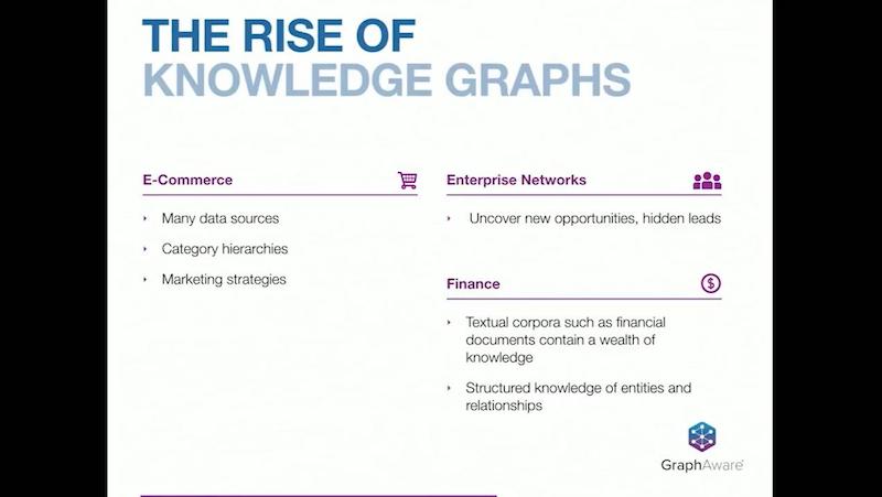
Knowledge graphs have been on the rise for the last couple of years across industries and use cases.

Discover where knowledge graphs are most widely used today.

In ecommerce, you have multiple data sources. It is one of the primary use cases for knowledge graphs. There are multiple category hierarchies; you almost never have a single hierarchy of products. You have products that are part of multiple different hierarchies.

This is quite a difficult problem to address if you don’t have a graph database. You have the combination of not only products, categories, and data sources, but also marketing. Marketing strategies and promotions influence what you sell. The combination of these three elements merge well into the concept of a knowledge graph.

Enterprise networks connect partners, customers, employees, opportunities and providers. Knowledge graphs help you discover relationships between all these connected data sets and therefore discover new opportunities.

Finance has a textual corpora of financial documents, which contain a wealth of knowledge. There are many case studies such as the ICIJ’s use of Neo4j to analyze the Panama Papers, an analysis that linked together more than 11 million documents. You end up with a very structured graph of entities, and how they are connected.

Learn what industries are taking advantage of knowledge graphs.

Health is an important use case for knowledge graphs that has had many practical applications over the last few years. Knowledge graphs unify structured and unstructured data from multiple data sources and integrate them into a graph-based model with very dynamic ontologies where data is characterized and organized around people, places and events. This enables you to generate a lot of knowledge based on the co-occurrence of relationships and data.

Knowledge graphs are being used for uncovering patterns in disease progression, causal relations involving disease, symptoms and the treatment paths for numerous diseases. New relationships have been discovered that were previously unrecognized simply by putting all this data together and applying a context around where it happened, who was involved and other natural events that might have happened around this data.

Criminal investigation and intelligence is an area where numerous papers have been published recently about how knowledge graphs helped in investigating cases. One of the most familiar cases has been around the area of human trafficking. Knowledge graphs have helped, because it is a difficult field to track, and much of the information is obfuscated. Coded messages are posted on public forums and they form a pattern. Tools and techniques such as natural language processing (NLP) decode these messages, make sense of them, and apply context around them.

Another key part of the whole knowledge graph is that, especially with law enforcement, you really need to have traceability from your knowledge graph back to your source of information. Otherwise, none of this would hold up in a court of law. With the knowledge graph, you also maintain the traceability of your data from the source to the point at which it clearly provides you the information or the evidence that you need.

Data Sparsity


Now we’re going to talk about some of the problems you see around data sparsity.

Learn about the problems surrounding data sparsity.

When you talk about collaborative filtering, one of the classic problems is a cold start. You cannot really recommend products or things to other people if you don’t even have other people in your graph or other purchases in your graph. This is commonly solved through things like tagging-based systems or trust networks. If you don’t have collaborative filtering, even content-based recommendation suffers a lot of problems due to missing data or wrong data. If you don’t have an enhanced graph to put all this data together, these are hard problems to solve.

With text search as well, with sparse data, you end up with user agnostic searches, and the world is moving away from anonymous agnostic searches to relevant context-oriented searches. Similarly, relevant search is a problem. So, these are some of the areas that we’ll touch upon in the later part of the presentation.

Knowledge Bases on Steroids


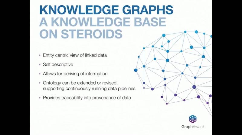
Knowledge graphs are what we used to know as knowledge bases but on steroids.

Learn why knowledge graphs are really just a knowledge base on steroids.

Knowledge graphs provide you an entity-centric view of your linked data. They’re self descriptive, because the data that’s described is really described in your graph.

Therefore, you’re capable of growing this data in an organic fashion, enhancing it as you discover more and more facts about your data. You have an ontology that can be extended or revised, and it supports continuously running data pipelines. It’s not a static system that’s once built, remains that way forever; it grows as your domain expands.

Back to the law enforcement use case, it provides you traceability into the provenance of data, and this is important in many industries.

Knowledge Graphs as Data Convergence


A knowledge graph is really a convergence of data from a variety of places (see below).

Discover how a knowledge graphs is a convergence of data.

You have data sources, which could come from all over the place, in all sorts of formats. You have external sources to enrich the data you have. You have user interaction, so as users play with your application or your domain, you learn more, you feed it back into the knowledge graph, and, therefore, you improve your knowledge graph. You have tools such as machine learning processes or NLP, which really, in the end, help you achieve your business goals.


Alessandro Negro: Let’s consider a specific application of knowledge graphs – a specific use case that implements an advanced search engine that delivers relevant search capabilities to the end user.
Learn how a knowledge graph provides relevant search capabilities.

Relevance here is the practice of improving search results, satisfying your data information needs in the context of a very specific user experience while combining or balancing how ranking impacts on a business’ certain needs.

Let’s walk through an implementation that combines graphs and, specifically, knowledge graphs, with Elasticsearch in order to deliver services to the end user.

You will see a real architecture and a concrete infrastructure where, combining both, it’s possible to deliver a high-level set of services to the end user. You will notice how knowledge graphs could help in this direction, not only because they solve issues related to data sparsity, but also because graphs represent a direct model for delivering these types of services to the end user.

Four Dimensions of Relevant Search


According to the definition stated before, relevance moves along four different dimensions. It revolves around four different elements: text, user, context and business goal.

Check out the dimensions of relevant search.

First of all, a search has to satisfy an information need that is expressed by the user using a textual query.

So, in this context, information retrieval and natural language processing are key to provide search results that mostly satisfy the user intent expressed by the search query. But relevant search moves toward a more user-centric perspective of the search. That means that we can’t deliver the same result set to the same user even if they perform the same query.

In this way, user modeling and the recommendation engine could help to customize the result set according to the user profile or the user preferences. While on the other hand, context expresses the special conditions under which that specific search has been performed. Contextual information like location, time, or even the weather could be helpful to further refine the search results according to the needs of the user while he was performing the query.

Last but not least, the business goals drive the entire implementation, because a search exists only to satisfy a specific need of an organization in terms of revenue or in terms of a specific goal that it would like to achieve. Moreover, a relevant search has to store a lot of information related to search histories or feedback loops. And all this data has to be accessed in a way that shouldn’t affect the user experience in terms of performance that will impact response time or the quality of the results.


Here is where knowledge graphs come in, because we will see how knowledge graphs represent the right approach in terms of information structure for providing relevant search.

See how to structure information for relevant search.

In order to provide a relevant search, a search architecture has to handle high quality, high quantity of data that is heterogeneous in terms of schemas, sources,volume, and rate of generation. Furthermore, it has to be accessed as a unified data source. That means that it has to be normalized and accessed as a unified schema structure that satisfies all the informational and navigational requirements of a relevant search that we saw before.

Graphs are the right representation for all the issues related to relevant search including information extraction, recommendation engines, context representation, and even a rules engine for representing business goals.

Information extraction attempts to make the semantic structure in the text explicit, because we refer to text as unstructured data, but text has a lot of structure related to the grammar and the constraints of the language.

You can extract this information using natural language processing. From a document, you can extract the sentences. And for each sentence, you can extract a list of tags. And then, the relationships between these tags based on the types of dependencies, mentions or whatever else.

This is a connected set of data that can be easily stored in a graph. Once you store this data, you may easily extend the knowledge that you have about it, ingesting information from other knowledge graphs like ConceptNet 5, which is an ontology structure that can be easily integrated in this basic set of information, adding new relationships to the graph.

On the other hand, recommendation engines are also built using user-item interactions that are easily stored in a graph. They can also be built using a content-based approach in which you will need to use informational extraction or a description or a list of features of the element you would like to recommend.

In both cases, the output of the process could be a list of similarities that could be easily stored in a graph as new relationships between items or between users. And then, you could use them to provide recommendations to the user that combine both approaches.

Context, by definition, is a multidimensional representation of a status or an event. Mainly, it is a multidimensional array. It is a tensor. A tensor is easily represented in a graph where you have an element that is one node and all the other indexes that refer to that element are other nodes that point to that specific node.

In this way, you can easily perform any sort of operation on the tensor, such as slicing, for example, or whatever else. Even easier is adding new indexes to this tensor – just adding a new node that points it to the element.

Finally, in order to apply a specific business goal, you have to implement a sort of rule engine. And even in this case, a graph could help you not only to store the rule itself, but also to enforce the rule in your system.

Use Case: Ecommerce Search Engine


Let’s consider a specific use case: a search engine for an ecommerce site.

Check out this knowledge graph use case for ecommerce.

Every search application has its own requirements and its own dramatically specific set of constraints in terms of expectations from the search. In the case of a web search engine, you have millions of pages that are completely different from each other. And even the source of the knowledge cannot be trusted.

You might think ecommerce search is a simpler case, but it is not. It’s true that the set of documents is more controlled and in terms of numbers, reduced. But in an ecommerce site, the categories of navigation and the text search are the main “salespeople,” not just a way for searching for something. They also a way for promoting something, for shortening path between the need and the buyer. They are very important.

In terms of expectations, a search in an ecommerce site has a lot of things to do. But even more, in this case, you can gather data coming from multiple data sources: sellers, content providers, and marketers pushing a strategy or marketing campaign in the system like promotions, offers, or whatever else.

Also, you have to consider the users. You have to store user-item interactions and user feedback in order to customize the results provided to the user according to their history. And obviously, again, there are business constraints.

Here is a simplified example of a knowledge graph for an ecommerce site:

Check out this simplified example of a knowledge graph for ecommerce.

The main element, in this case, is represented by the products. Here we have just three products: an iPhone, a case for the iPhone, and an earphone. For every product, we have some information like the list of features that describe that product. But obviously this list of features will change according to the type of the product, so it will be different for a TV, a pair of shoes and so on.

Starting from this information, it’s easy to process the textual description and the list of tags. Once we have the tags, we are able to ingest data from ConceptNet 5 and know that a smartphone is a personal device.We will see how this is valuable information later on for providing relevant search. But apart from the data that is common for this type of application, we also analyze our data and create new relationships between items.

This is how relationships like “usually bought together” come into play. It’s also possible to manually add relationships, like the relationship between a phone and a case. In this way, you are augmenting the amount of knowledge that you have step by step and using all this knowledge during the search and during catalog navigation.

Infrastructure for the Knowledge Graph


With all these ideas in mind, we designed this infrastructure for one of our customers:

Check out GraphAware's knowledge graph infrastructure using Neo4j and Elasticsearch.

The knowledge graph is the main source of truth in this infrastructure, and several other sources feed the knowledge graph. A machine-learning platform processes the graph continuously and extracts insights from the knowledge graph and then stores the insights back into the knowledge graph.

Later we’ll discuss how the integration with Elasticsearch allows us to export multiple views with multiple scopes so that knowledge graph queries do not impact the front end too much. We use Elasticsearch as a sort of cache and also a powerful search engine on top of our knowledge graph.

Data Flow for the Knowledge Graph


For the data flow, we designed an asynchronous data ingestion process where we have multiple data sources pushing data in multiple queues. A microservice infrastructure reacts to these events, processes them, and stores this intermediate data in one queue that then is processed by a single Neo4j Writer element that reads the data and stores it in the graph.

This avoids any issues in terms of concurrency, and it also enables us to easily implement a priority-based mechanism that allows us to assign different priorities to an element.

Storing Multiple Views in Elasticsearch


In order to store multiple views in Elasticsearch, we created an event-based notification system that is highly customizable and capable of pushing several types of events. The Elasticsearch Writer reacts to these events, reads data from the knowledge graph and creates new documents or updates existing documents in Elasticsearch.

The Role of Neo4j


Neo4j is the core of this infrastructure because it stores the knowledge graph, which is the only source of truth. There is no other data somewhere else. All the data that we would like to process is here. It all converges here in this knowledge graph.

Learn about Neo4j's role in the knowledge graph.

Neo4j is a valuable tool because it allows you to store several types of data: users, products, details about products and whatever else. It also provides an easy-to-query mechanism and an easy-to-navigate system for easily accessing this data.

More than that, in the early stage of the relevant search implementation, it can help the relevance engineer to identify the most interesting feature in the knowledge graph that’s useful for the implementation of the related search in the system.

Moreover, once all the data is in the graph, it goes through a process of extension that includes three different operations: cleaning, existing data augmentation and data merging. Because multiple sources can express the same concept in different ways, data merging is also important.

Machine Learning for Memory-Intensive Processes


Some of these processes can be accomplished in Neo4j itself with some plugins or with Cypher queries. Others need to be externalized, because they are intensive in terms of computational needs and memory requirements.

We created a machine learning platform (see below) that, thanks to the Neo4j Spark connector, allows us to extract data from Neo4j, process it using natural language processing or even recommendation model building, and then store this new data in Neo4j, which will be useful later on for providing advanced features for the relevant search.

Discover more about enternalise intense processes.

Elasticsearch for Fast Results


We are trying to use the right tool for the right job. We use Neo4j for storing the knowledge graph and it is perhaps the most valuable tool for doing this, but obviously, in terms of textual search, it could be an issue if you want to perform more advanced textual search in Neo4j. We added Elasticsearch on top of Neo4j in order to provide fast, reliable, and easy-to-tune textual search.

Learn more about Elasticsearch roles in the knowledge graph.

We store multiple views of the same data set in Elasticsearch for solving several scopes and for serving several functionalities that are faceting. Faceting means any sort of aggregation of the result set that you want to have. You can serve a product details page or provide product variants aggregation. With Elasticsearch, you can also provide auto-completion or suggestions.

Elasticsearch is not a database, and we don’t want to use it as a database. It is just a search engine for data from Neo4j in this use case and is a valuable tool for textual search.

Relevant Search on Top of Knowledge Graph


Now let’s explore using Elasticsearch to provide relevant search on top of the knowledge graph that we built using the infrastructure covered earlier.

What Is a Signal?


In terms of relevant search, a signal is any component of a relevance-scoring calculation corresponding to meaningful and measurable information. At its simplest, it is just a field in a document in Elasticsearch.

The complicated part is how you design this field, what you put inside it and how you can extract from the knowledge graph and store data in Elasticsearch that really matters.

There are two main techniques for controlling relevancy (see below). The first one is signal modeling. It is how you design the list of fields that compose your documents in order to react to some textual query. And the other one is the ranking function, or the ranking functions, that are how you compose several signals and assign each of them a specific weight in order to obtain the final score and the rank of the results.

Learn more about crafting signals in the knowledge graph.

You always have to balance precision and recall where, in this context, precision is the percentage of documents in the result set that are relevant and recall is the percentage of relevant documents in the result set.

It’s a complicated topic, but to simplify it, if you return all the documents to the user, you have a recall of 100%, because you have all the relevant documents in the result set. With a recall of 100%, you have a very low degree of precision. And even in this case, you can have multiple sources in terms of data from the knowledge graph that you can use for modeling your signal.


Let me give you a couple of examples. The first approach is personalizing search.

Learn more about personalizing search with a knowledge graph.

Here, we include users as a new source of information so we can provide a customized result set. We would like to customize the result set according to the user profile or the user preferences.

We have two different approaches. The first one is a profile-based approach where we create a user profile that could be created manually by the user by filling out a form, or automatically, inferring user preferences from past searches.

The second approach is behavioral based. In this case, it’s more related to a recommendation engine that analyzes the user-item interaction in order to make explicit the relationship among users and items.

Once you have a user profile or behavioral information, you have to tie this information to the query. And you can do this in three different ways: at query time, changing the query according to the recommendation that you would like to make; at index time, changing the documents according to the recommendation that you would like to make; or using a combined approach.

For example, if you would like to customize the results for the user at query time, you have to change your query, specifying the list of products that the user may be interested in. In this way, you could easily boost the results if the results set includes some of the products that the user is known to be interested in. On the other hand, at index time, you would have to store a list of users that may be interested in each product. And then you can easily boost results that specifically match in that case.


Another interesting extension of the classical search is the concept search. In this case, we move from searching for strings to searching for things.

Discover how a knowledge graph assists with concept search capabilities.

The user could use different words for expressing the same concept. This can be an issue in a classical text search environment where you have to match the specific word that appears in the text. Using the techniques that we described before in terms of data enrichment, you can easily extend the knowledge that you have about each word. You can easily store those words in Elasticsearch and react to the user’s query even if he is not using the terms that are on the page.

There are different approaches to enriching this information. You can manually, or even automatically, add a list of tags that could be helpful in terms of the describing the content. You can write a list of synonyms. For example, for TV, you can have synonyms like T.V., or television, or whatever else. And in this way, even if the text says TV, you can easily provide results if the user writes television, for example.

There is a more advanced approach in which you use machine learning tools for augmenting the knowledge. You can use a simple co-occurrence as well as Latent Dirichlet Allocation. That means clustering your document set, and finding the set of the words that better describes that specific cluster and all the documents in that cluster.

Combining Neo4j and Elasticsearch: Two Approaches


Here are two different approaches that we tried when integrating Neo4j and Elasticsearch.

On the left side below is the first approach, which has two elements: the documents in Elasticsearch and the graph database.

Discover combined search approaches for the knowledge graph.

In this approach, when a user performed a query, it goes through two different phases. The first one is the classical textual search query that is performed entirely on Elasticsearch.

The first result set is then manipulated by accessing the graph, and boosting the results according to whatever rule you’d like to use. This approach could work, but in terms of performance, could suffer a little bit when you have to do complex boosting operations.

As a result, we moved to the second approach (see above right), in which there is a tighter connection between Elasticsearch and the knowledge graph. Using this approach, as discussed earlier, the knowledge graph is used for exporting multiple views into Elasticsearch.

Part of the work is done at index time. When the user performs a query, the query itself goes through a first stage that is an enrichment. Accessing the graph, we can change the query, and then we perform the query against Elasticsearch. This appears to be a more performant approach, because this operation itself is not related to every single element in the graph, but is narrowed based on the context or on the user, so it is very fast.

We can use Elasticsearch for what is supposed to be just textual search. But at that point, we already have a very complex query that is created using the graph. And even the indexes are really changed according to the graph’s structure.

Conclusion

Knowledge graphs are very important because they use graphs for representing complex knowledge. Knowledge graphs use an easy-to-query model that allows us to gather data from several sources. That means we can store users, user-item interactions, and whatever else we want. We can further extend important data later on or change our knowledge graph by adding new information.

On top of this, we can implement a search engine like Elasticsearch, which is fast, reliable, and easy-to-tune and which provides other interesting features, such as faceting and auto-completion.

By combining Neo4j and Elasticsearch, you can deliver a high level set of services to the end user. The takeaway is to use the right tool for the right job. You can use a graph for representing complex knowledge and a simple tool like Elasticsearch to provide textual search capability and advanced search capability to the end user.


Level up your recommendation engine:
Learn why a recommender system built on graph technology is more powerful and efficient with this white paper, Powering Recommendations with Graph Databases – get your copy today.


Read the White Paper

Graphs in Government: Introduction to Graph Technology

$
0
0
Discover how graph technology is being used in government.
The use cases for a graph database in government are endless.

Graphs are versatile and dynamic. They are the key to solving the challenges you face in fulfilling your mission.

Using real-world government use cases, this blog series explains how graphs solve a broad range of complex problems that can’t be solved in any other way.

Discover how graph technology is being used in government.

In this series, we will show how storing data in a graph offers benefits at scale, for everything from the massive graph used by the U.S. Army for managing strategic assets to recalling NASA’s lessons learned over the past 50 years.

Graphs Are Everywhere


Everywhere you look, you’ll find problems whose solutions involve connecting data and traversing data relationships, often across different applications or repositories, to answer questions that span processes and departments.

Uncovering the relationships between data locked in various repositories requires a graph database platform that’s flexible, scalable and powerful. A graph database platform reveals data connectedness to achieve your agency’s mission-critical objectives – and so much more.

The Power of a Graph Database Platform


To understand the power of a graph database, first consider its collection-oriented predecessor, a traditional relational database.

Relational databases are good for well-understood, often aggregated, data structures that don’t change frequently – known problems involving minimally connected or discrete data. Increasingly, however, government agencies and organizations are faced with problems where the data topology is dynamic and difficult to predict, and relationships among the data contribute meaning, context and value. These connection-oriented scenarios necessitate a graph database.

A graph database enables you to discover connections among data, and do so much faster than joining tables within a traditional relational database or even using another NoSQL database such as MongoDB or Elasticsearch.

Neo4j is a highly scalable, native graph database that stores and manages data relationships as first-class entities. This means the database maintains knowledge of the relationships, as opposed to a relational database (RDBMS), which instantiates relationships using table JOINs based on a shared key or index.

A native graph database like Neo4j offers index-free adjacency: data is inherently connected with no foreign keys required. The relationships are stored right with the data object, and connected nodes physically point to each other.

Discover the difference between a relational database and a graph database.


Conclusion


As we’ve shown, a graph database enables you to discover connections among data, and do so much faster than joining tables within a traditional relational database.

Graph databases are as versatile as the government agencies that use them. In the coming weeks, we’ll continue showing the innovative ways government agencies are using graph databases to fulfill their missions.


Solutions can’t wait:
Witness how leading government agencies are using Neo4j to overcome their toughest challenges with this white paper, Graphs in Government: Fulfilling Your Mission with Neo4j. Click below to get your free copy.


Read the White Paper


Google Kubernetes Engine and Neo4j: Power Your Apps with Graphs

$
0
0
Learn about Google Kubernetes and Neo4j.
Google Kubernetes Engine (GKE) is a hosted, managed version of Kubernetes. As such, it is a great environment for developers to start experimenting with the many use cases for Neo4j. Neo4j is available through the Google Cloud Platform Marketplace, so developers familiar with Kubernetes can have Neo4j running in minutes.

In this series, we will explore the power of containers and Kubernetes in combination with Neo4j. This week we’ll provide some background about Kubernetes and Neoj.

Learn about Google Kubernetes and Neo4j.


Power of Containers + Kubernetes


You probably already know the value of containers – and using Kubernetes to manage those containers – but here’s a brief recap.

Containers enable you to package an application and all of its dependencies, making the workload portable and eliminating the need to install or configure software. Instead of installing software on servers, users simply drop a container in place and tell the server to execute that software.

Once users see the value of containers, they tend to deploy them more widely. Users develop complex workloads that involve multiple containers talking to one other. They build larger architectures that involve a number of different applications in containers, which increases the management challenges they face. All of those containers must work together (that is, they must be orchestrated). That’s where Kubernetes comes in.

Kubernetes, originally developed by Google, is an open source container orchestration platform released in 2014. Since then, Kubernetes has become the de facto standard for container orchestration. For example, you may have a fleet of containers running on a number of physical servers; Kubernetes schedules those containers onto the appropriate servers. As container deployment becomes more complicated, Kubernetes orchestrates many different container workloads across a cluster of physical machines according to policies that you define.

More Power with GKE


The operational overhead of setting up, configuring and managing Kubernetes is challenging.

Enter Google Kubernetes Engine (GKE). GKE is Kubernetes hosted and managed for you – better, easier and more affordably than you can manage yourself – and with the added powerful benefits of scalability and uptime guarantees.

With GKE, you easily run flexible business workloads and connect those workloads. GKE enables you to run a wide variety of applications and services, including persistent storage and databases. With GKE, your container architecture operates seamlessly with high availability. Google Site Reliability Engineers (SREs) constantly monitor your cluster and its compute, networking and storage resources so you don’t have to – giving you back time to focus on your applications.

Application Deployment Made Easy: Google Cloud Platform (GCP) Marketplace


GKE is Kubernetes, expertly managed and simplified for you. All you need now is an app store. The GCP Marketplace features numerous applications and components for you to easily deploy. You may have heard of graph database like Neo4j or have even thought of experimenting with them but don’t know where to start. The GCP Marketplace removes the friction of deployment and orchestration. That way you’re up and running within minutes on GKE when you utilize applications like Neo4j Enterprise Edition or its Causal Clustering features.

The Power of a Graph Database Platform


Despite what’s implied in the name, relational databases (RDBMS) don’t excel at identifying relationships among data.

While relational databases manage volumes of information, they lack the ability to generate insight from that data. The value of data increases exponentially when it’s connected and its relationships are revealed – which is where a graph database comes into play.

A graph database enables you to query your data and discover connections and relationships among data much faster than JOINing tables within a traditional relational database or even using another NoSQL database such as MongoDB or Elasticsearch.

Neo4j is a highly scalable, native graph database that stores and manages data relationships as first-class entities. The graph data model is easy to understand because it reflects how data naturally exists – as objects and the relationships between those objects. It’s a model that you naturally sketch on a whiteboard when talking about data, with data elements (nodes) and the relationships between them.


Conclusion


Neo4j helps you solve connected data problems with high performance and flexibility. GKE manages all of your infrastructure and gives you best-in-class cloud capabilities.

Next week, we’ll dive deeper into the specific benefits of deploying Neo4j on GKE and how Google Cloud Platform Marketplace brings the two together to help you get started in minutes.


Get started with Google Kubernetes Engine and Neo4j
See how developers are adding graph superpowers to their applications in this white paper, How GKE and Neo4j Power Your Apps with Graphs. Click below to get your free copy.


Read the White Paper


Importing Data from the Web with Norconex & Neo4j

$
0
0
Get down into the details of important data from the web with Norconex and Neo4j.


Neo4j provides many tools for importing data, such as LOAD CSV (from Cypher queries) and the neo4j-admin import tool.

It is also possible to import data from many other systems like ElasticSearch, SQL databases, MongoDB, and CouchBase (using an APOC procedures plugin).

Finally, ETL tools like Kettle provide features, which aims the effort needed for the data transformation. In short, the data manipulation ecosystem around Neo4j is very nearly complete.

To add another facet to this ecosystem, we present a way for Neo4j to obtain data directly from the web. To do this we use an external tool called a Web Crawler (also known as a Web Spider or a Web Scraper).

What Is a Web Crawler?


A Web Crawler is a robotic program which specializes in browsing the web, digging more and more deeply by following links. The basic operation is pretty simple.

Consider the following cycle of work:

    • Download a webpage
    • Extract the links from this page to other pages and add them to the frontier (a pool of URLs)
    • Extract content and meta-data from this page and store it somewhere


Caution: Politeness Rules


While it’s true that the basic principle of crawling is simple, to be a good internet citizen you must respect politeness rules. This is really important – ​we don’t want to end up attacking a website, we just want to grab useful data!

Here are some politeness rules:

    • Provide a think time, that is a time delay between two hits. This gives the target host some time to catch its breath. Also avoid hitting a site with more than one thread.
    • Respect site rules contained in ROBOTS.TXT files and nofollow directives.
    • Be careful not to download personal data.
If you are impolite, you risk being blacklisted, or, worse, to knock over the remote server. This is clearly not a good way to treat a site whose data we need!

Norconex Web Crawler


Norconex is an IT company located in Gatineau, Quebec, Canada, which specializes in enterprise internet searches. Norconex provides a very nice open source Web Crawler, known as HTTP Collector. The Norconex crawler is, in essence, a generic pluggable crawl engine.

Take a look at its structure on the image below:


Many collectors are provided by Norconex (HTTP, FileSystem, etc.) In addition many connectors, called committers, are provided which inject data (SQL, ElasticSearch, Solr, etc.).

Using a simple XML configuration, you can connect an input (a data collector) to an output (a committer). You can also apply filters or perform data transformation between the collector and the committer.

The newest committer is the Neo4j committer.

Meet the California Grapes


I live in Burgundy, France, and I have enjoyed tasting many wines from this region (as well as from other regions in France). Especially important are the Pinot Noir grape, for red wines, and the Chardonnay grape for white wines.

There is an interesting wine history between the New and Old Worlds. Many European grape varietals were exported from Europe to the United States. This was of critical importance because in the 19th century the Phylloxéra aphid plague wreaked havoc, damaging vineyards on the European continent (especially France). The French grapes were ultimately saved using greffons from American foot vines.

Despite this historical connection, I don’t really know much about American wines. After reading an article, I decided I should introduce myself to California wines (which make up about 90% of American wine production).

Okay, let’s go to meet the California grapes.

Norconex Considerations


A crawl is configured by XML. Consider the following points:

    • Metadata is the information placed in the <head/> section of the HTML page, plus some information added by the Norconex engine (as collector.referenced-urls, which stores all the links available on this page). This data is stored as key/value pairs.
    • Content is the main content placed in <body/> section of the HTML page.
You can see the flow of the HTTP Collector here: https://www.norconex.com/collectors/collector-http/flow.

Finding Sources


After searching the internet, I found a good start point: https://discovercaliforniawines.com/.

It contains data about regions, sub-regions, wineries and grapes. My goal is to build a graph with the data to display how each grape varietal is divided over the regions or sub-regions.

After some site analysis, I decide to split this work in two crawls:

    • Importing varietals first (one XML configuration)
    • Importing regions, sub-regions and wineries then (another XML configuration)
Later, I’ll probably need to wash the data to eliminate noise nodes (unwanted nodes or relationships).

Import Grape Varietals


Starting with Sources (Start URLs)


By inspecting the source code for this page: https://discovercaliforniawines.com/wine-map-winery-directory/, I find there is a search selector which lists all the kinds of grapes, the text values being the grape names and the option value attribute being the IDs.

I’ll begin the XML configuration by specifying the starting URLs:

<startURLs stayOnDomain="true" stayOnPort="true" stayOnProtocol="true">
      <url>https://discovercaliforniawines.com/wine-map-winery-directory/</url>
</startURLs>

Making One Document Too Many


Norconex is able to split one document into many documents, based on a CSS selector. This way I can split each option on this <select/> tag:

 <importer>
        <preParseHandlers>
          <splitter class="com.norconex.importer.handler.splitter.impl.DOMSplitter"
            selector="#varietal_select option"
            parser="html"/>

The importer phase is reached when the document (the Web page) passes through filters, and then the document treatment process begins. Here, the DOMSplitter component makes one document (imported as new document) for each tag matching the CSS selector #varietal_select option.

Adding value and id


Each new document content built by the DOMSplitter looks like (as an example):

<option class="text-dark" value="1554">Cabernet Sauvignon<option>

It will be useful to extract the text value and id to put them in the metadata. As we will see later, the varietal can then be linked to wineries with this identifier.

Norconex provides a component to extract data from CSS Selector, the DOMTagger:

          <tagger class="com.norconex.importer.handler.tagger.impl.DOMTagger">
              <dom selector="option"  toField="varietal_id"   extract="attr(value)"/>
              <dom selector="option"  toField="varietal"   extract="ownText"/>
          </tagger>

Stamping These Pages with Varietal Type


To provide more qualified information when the document will be stored to Neo4j (see the Additional Labels section beloow), we’re going to add a constant on each page imported from the document splitter.

Norconex provides a ConstantTagger to add a explicit value to a metadata field—​here the field is TYPE:

          <tagger class="com.norconex.importer.handler.tagger.impl.ConstantTagger"
              onConflict="replace" >
            <restrictTo caseSensitive="false" field="document.embedded.reference">
               #varietal_select.*
            </restrictTo>
           <constant name="TYPE">VARIETAL</constant>
          </tagger>

      <preParseHandlers>
   <importer>

The restrictTo element allows us to provide a regular expression to filter the documents tagged.

Storing in Neo4j


The ultimate goal is to store the data in Neo4j.

First of all, we choose the committer Norconex provides for Neo4j: com.norconex.committer.neo4j.Neo4jCommitter

This committer must be configured with the following information:

    • The Neo4j connection information
    • The node topology (SPLITTED, ONE_NODE, NO_CONTENT)
    • The primary label
    • The additional labels (optional)
    • The relationships definitions (optional)
Other configuration information is mostly common to all the other Norconex committers.

	<committer class="com.norconex.committer.neo4j.Neo4jCommitter">
		<uri>bolt://localhost:7687</uri>
		<user>neo4j</user>
		<password>neo4j</password>
		<authentType>BASIC</authentType>

		<nodeTopology>NO_CONTENT</nodeTopology>
		<primaryLabel>CALIFORNIA</primaryLabel>

		<additionalLabels>
			<sourceField keep="true">TYPE</sourceField>
		</additionalLabels>

		<sourceReferenceField keep="true">document.reference</sourceReferenceField>
		<targetReferenceField>identity</targetReferenceField>

		<queueSize>5</queueSize>
	</committer>

Node Topology

The node topology defines how a Web page must be stored in Neo4j:

    • ONE_NODE: the page will be stored in one node which contains metadata and content
    • NO_CONTENT: the page will be stored in one node which contains only metadata
    • SPLITTED: the page will be stored in three nodes, one super node linked to another one which contains metadata and linked to another one which contains content
In my case, I’m not interested in the content – ​I want only to know how the entities are linked. So I chose the NO_CONTENT topology.

Primary Label

All nodes imported by this crawl will be stamped with a label by this literal value. This makes it easy to delete or search only on them.

Additional Labels

Additional labels are used to define the nodes more precisely. Here we need to parameterize a metadata field. The value of this key will be converted into a label on the node.

Remember that earlier a constant, named TYPE, was configured with the ConstantTagger. This is the value I want to add to new nodes.

Starting Norconex and Check the Result


Now my configuration is completed, I can launch the Web crawler:

$> sh collector-http -a start -c confs/california-varietals.xml

    • -a: the action, start or stop
    • -c: the config file path
When it finishes I can check the imported Neo4j data:

MATCH (v:VARIETAL) RETURN v.varietal, v.varietal_id

And the query produces the following result:


As we can see, we’ve gotten some unwanted data, that is All Varietals. This is because it was the first value in the varietal selector on the web page. We can clean up this data by deleting all nodes where varietal_id is null:

MATCH (v:VARIETAL) WHERE v.varietal_id IS NULL DELETE v

Import Regions and Sub-Regions


Start URL and Link Extractor


Now I want to import the California regions and their sub-regions. This website has a page at https://discovercaliforniawines.com/discover-california/. This page has a sub-banner with links to all the regions (North Coast, Central Coast, etc). And on each page of these regions, there are the links to sub-regions (Lake Country, Los Carneros, etc.). Nice.

My starting URL will be https://discovercaliforniawines.com/discover-california/ but I don’t want to extract all links from this page, because there are links to thing that are not useful for my purposes, such as links to events, media, etc.

So, I really only want to extract links from the sub-banner with the CSS selector #page-menu-bar. This will also reduce the processing time.

Norconex allows us to modify the default behavior of its link extractor like this:

	<linkExtractors>
		<extractor class="com.norconex.collector.http.url.impl.GenericLinkExtractor">
			<extractSelector>#page-menu-bar</extractSelector>

		</extractor>
	</linkExtractors>

Note: There are many other parameters for the GenericLinkExtractor and other usages, too.

Reference and Document Filters


We need to say a bit here about filters. The reference filters are based on the extracted links, whether or not we put them into the frontier. Document filters are triggered when the document is downloaded, and filtering is based on the document’s meta-data or content.

Our filters are using the Norconex RegexReferenceFilter, a filter based on the reference of the document or its link:

	<filter class="com.norconex.collector.core.filter.impl.RegexReferenceFilter" onMatch="include">
      		https://discovercaliforniawines.com/discover-california/.*
        </filter>

Constant TYPE for Additional Labels


As we did with varietal, we need to qualify our new nodes more precisely:

	<tagger class="com.norconex.importer.handler.tagger.impl.ConstantTagger"
              onConflict="noop" >
            <restrictTo caseSensitive="false" field="document.reference">
                https://discovercaliforniawines.com/discover-california/[\w-?]*/?{0,0}
            </restrictTo>
            <constant name="TYPE">CALIFORNIA_REGION</constant>
        </tagger>
        <tagger class="com.norconex.importer.handler.tagger.impl.ConstantTagger"
              onConflict="noop" >
            <restrictTo caseSensitive="false" field="document.reference">
                https://discovercaliforniawines.com/discover-california/[\w-?]*/.*
            </restrictTo>
            <constant name="TYPE">CALIFORNIA_SUB_REGION</constant>
        </tagger>

Neo4j Committer: Creating the Relationships


Creating the Neo4j relationships is probably the most difficult and interesting part of a configuration. It is also essential because relationships are crucial to the graph.

First of all, we want to link regions to their sub regions. A region HAS a sub region. Each time we parse a CALIFORNIAREGION tagged document, we want to create a relationship to a CALIFORNIASUBREGION with the relationship type HASSUB__REGION. Take a look at the following configuration:

	<relationships>
		<relationship type="HAS_SUB_REGION" direction="OUTGOING" targetFindSyntax="MERGE" regexFilter="https://discovercaliforniawines.com/discover-california/[\\w-?]+/.+">

			<sourcePropertyKey label="CALIFORNIA_REGION">collector.referenced-urls</sourcePropertyKey>
		 	<targetPropertyKey label="CALIFORNIA_SUB_REGION">identity</targetPropertyKey>
		</relationship>
	</relationships>


    • The type attribute is the name of the Neo4j’s relationship.
    • The direction attribute denotes its sense.
    • The targetFindSyntax gives the way the Cypher query is to be created with these parameters. With MATCH, if the targeted node doesn’t exist, then the relationship will not be created; with MERGE, if the targeted node doesn’t exist, it will be created.
    • The regexFilter attribute allows us to apply the relationship only on the pages where The source property value (see below) matches the regex. This will avoid linking spurious nodes.
The following elements are:

    • sourcePropertyKey: to define constraints for building the relationship from the current committed page
    • targetPropertyKey: to define the concerned nodes that should be linked
The label attribute is an optional constraint, and in this case each node source or target (or both) must have the requisite label.

Finally, the value inside the element will be evaluated from a meta-data property (for source) and from a node property (for target). If the source value is multi-valued (like collector.referenced-urls) then one relationship could be created for each value.

To summarize, each URL in the source meta-data property collector.referenced-urls which matches the regex filter is going to create a relationship with a target which has a property identity (default id if not otherwise specified in the document.reference, it will default to the page url) when a match occurs. If there is no match, the target node is created (because we set targetFindSyntax="MERGE") with the provided identity and the label specified by the constraint in the target node. The targeted node will be completed later when the crawler reaches the concerned pages.

Linking Sub-Regions with Grape Varietals Through Wineries


We have no way to link sub-regions to varietals directly. On this web site, varietals are only referenced by wineries. But we can first link sub regions to wineries and then link wineries to varietals.

Importing Wineries


Importing wineries is not so easy, because there are redirections between sub-region pages to wineries pages. For example the link https://discovercaliforniawines.com/wineries/acorn-wineryalegria-vineyards-2/ from the sub-region page is redirected to https://discovercaliforniawines.com/wine-map-winery-directory/#winery=1393050&search=ACORN%20Winery%2FAlegr%C3%ADa%20Vineyards. To handle this situation and to get a continuous linkage between these pages, we’ll need to link them.

First, tagging nodes for TYPE:

<tagger class="com.norconex.importer.handler.tagger.impl.ConstantTagger"
            onConflict="noop" >
   <restrictTo caseSensitive="false" field="document.reference">
      https://discovercaliforniawines.com/wineries/.*
   </restrictTo>
   <constant name="TYPE">WINERY_REDIRECTION</constant>
</tagger>

<tagger class="com.norconex.importer.handler.tagger.impl.ConstantTagger"
            onConflict="noop" >
    <restrictTo caseSensitive="false" field="document.reference">
       https://discovercaliforniawines.com/wine-map-winery-directory/.+
    </restrictTo>
    <constant name="TYPE">WINERY</constant>
 </tagger>

Then, I’m going these specify this kind of node via the property redirect-trail on the targeted page metadata (which is injected by Norconex). We can do this by:

<relationship type="REDIRECT_TO" direction="INCOMING" targetFindSyntax="MATCH">
   <sourcePropertyKey label="WINERY">collector.redirect-trail</sourcePropertyKey>
   <targetPropertyKey label="WINERY_REDIRECTION">identity</targetPropertyKey>
</relationship>

This configuration leads the creation of links between nodes like: (wineryUrlFromSubregion)-[:REDIRECTED_TO]-(wineryLink)

Linking Sub-Regions


Having done this, the rest is pretty simple. Because we couldn’t link the CALIFORNIA_SUB_REGION nodes to WINERY nodes, we have to link the CALIFORNIA_SUB_REGION to WINERY_REDIRECTION nodes.

<relationship type="HAS_WINERY" direction="OUTGOING" targetFindSyntax="MERGE" regexFilter="https://discovercaliforniawines.com/wineries/.+">
   <sourcePropertyKey label="CALIFORNIA_SUB_REGION">collector.referenced-urls</sourcePropertyKey>
   <targetPropertyKey label="WINERY_REDIRECTION">identity</targetPropertyKey>
</relationship>

Note: the region “Far North California” doesn’t have a sub-region, and to make this article more readable, the relationship configuration is not shown here. But it is available in the full configuration (see Resources below).

Linking Varietals


Creating varietals links comes with a bit of complexity. To link a winery to matched varietal, we have to extract the varietal Ids from data on the page https://discovercaliforniawines.com/wine-map-winery-directory/. The winery selector has a lot of data like varietals-id. Using javascript, we can extract these varietals Ids and put them in the winery meta-data, with a new field called varietals:

<tagger class="com.norconex.importer.handler.tagger.impl.ScriptTagger">
             <restrictTo caseSensitive="false" field="document.reference">
             https://discovercaliforniawines.com/wine-map-winery-directory/.+
            </restrictTo>
            <script><![CDATA[
	        // extract winery id from URL
                var wineId =  reference.substring(
                    reference.indexOf("=") + 1,
                    reference.lastIndexOf("&")
                );
                metadata.addString('winery-id', wineId);

                // transform text content to Html DOM
                var jsoup = org.jsoup.Jsoup.parse(content);
		// retrieve element relative to current winery
                var elems = jsoup.getElementsByAttributeValue("data-id", wineId);
                var elem = elems.first();
                if (elem != null){
		  // extract data-varietals and transform array [] to | value separator
                  var varietals = elem.parent().attr("data-varietals");
                  varietals= varietals.replace("[","");
                  varietals= varietals.replace("]","");
                  var parts = varietals.split (",");
                  for (i = 0 ; i < parts.length ; i++){
                    metadata.addString('varietals', parts[i]);
                  }
                }
                else metadata.addString('varietals', 'none');

            ]]></script>
</tagger>

Now, we’re able to create the relationships from a winery to related varietals:

<relationship type="FROM_WINERY" direction="INCOMING" targetFindSyntax="MATCH">
   <sourcePropertyKey label="WINERY">varietals</sourcePropertyKey>
   <targetPropertyKey label="VARIETAL">varietal_id</targetPropertyKey>
</relationship>

Et voilà!

Note: labels filters on sourcePropertyKey and targetPropertyKey elements are not mandatory (because they are implicit in the graph). But, they are an easy way here to document the relationship.

Cleaning the Graph


Nice. I have a graph but this graph feels more like a crawl graph than a business graph. That is to say, we have many nodes that are artifacts of the Norconex web crawler download pages. For example, we don’t need the WINERY_REDIRECTION nodes at all anymore. So, we’ll clean up the graph by removing them and building relationships directly between subregions and wineries, via the following query:

MATCH (n)-[:HAS_WINERY]->(wr:WINERY_REDIRECTION)-[:REDIRECT_TO]->(w:WINERY)
DETACH DELETE wr
MERGE (n)-[:HAS_WINERY]->(w)

Querying the Graph


And now we can query the graph! First, we might like to know about the related regions and sub-regions:

MATCH (r:CALIFORNIA_REGION)
OPTIONAL MATCH (r)-[:HAS_SUB_REGION]->(sr:CALIFORNIA_SUB_REGION)
RETURN r.value AS Region, COLLECT(sr.value) AS Subregions


Next, say we want to know how many wineries are in each region:

MATCH (r:CALIFORNIA_SUB_REGION)-[:HAS_WINERY]->(w:WINERY)
RETURN r.value AS SubRegion, count(w) AS WineriesCount
ORDER BY WineriesCount DESC


Unsurprisingly, Napa Valley is at the top of the list. After all, Napa Valley is the only one American wine region I knew of up to now.

And finally, we can see how many types of wineries cultivate each kind of grapes:

MATCH (r:CALIFORNIA_REGION)
MATCH (r)-[:HAS_SUB_REGION]->(sr:CALIFORNIA_SUB_REGION)
MATCH (sr)-[:HAS_WINERY]->(w:WINERY)
MATCH (w)<-[:FROM_WINERY]->(v:VARIETAL)
WITH r,w, v ORDER BY v.value
RETURN v.value AS Varietal,COUNT(w) AS WineriesCount
ORDER BY WineriesCount DESC


We see that Cabernet Sauvignon is the most widely cultivated grape in California, at 329 wineries (out of 598). Cabernet Sauvignon is a red grape variety known worldwide, and it has become one of the most widespread grape varieties in the world. It owes its international recognition to the great wines from the vineyards of Bordeaux, France. Chardonnay, in second place, is a white grape from the vineyards of Burgundy, France. It is not only used to make great white wines but also to make sparkling champagne wines.

Beyond This Sample


This is certainly more interesting to work with winery surfaces instead of wineries count to really see what kind of grapes are the most cultivated. Also, with surfaces, we can find out what wineries are the most influential actor in a region. We can build a map to locate where the wineries are (and also compute a density). We might think about improving the varietal nodes by adding color or origin data, and by crossing this data with another crawl based on another web site which contains that kind of information. So you see, this sample could be extended to become a valuable data source about Californian wines.

Conclusion


Norconex and Neo4j make a powerful combination. Using the Neo4j Committer, we are able to grab linked data instead of data in the traditional table format. However, Norconex is also able to run many committers simultaneously, so we could imagine storing related data in Neo4j and content data (like text) in Elasticsearch in a single pass, for example.

Resources


All images in this article are built from Neo4j Bloom visualization tool: https://neo4j.com/bloom/

The Norconex configuration is based on Neo4j Committer v2: https://www.norconex.com/collectors/committer-neo4j/ and the Norconex Http-Collector v2.9.0-SNAPSHOT : https://www.norconex.com/collectors/collector-http/releases#a2.9.0-SNAPSHOT

You can find the two full configuration files here:

Special thanks to Frank Kutzler for reviewing.


Want to take your Neo4j skills up a notch? Take our online training class, Neo4j in Production, and learn how to scale the world’s leading graph database to unprecedented levels.

Take the Class
Viewing all 32 articles
Browse latest View live